CS189 Assignment1#
part2和part1其实差不多, 只是更深入的去实现一些机器学习的基本模型以及做一些图像增强的工作, 从算法难度上来说还不如part1里面那几个实现旋转变换的函数
Assignment Overview#
本部分代码位于fashion_pt_2.ipynb里面
加载MNIST数据集#
用torchvision调用api即可
# Load the FashionMNIST training dataset
train_data = torchvision.datasets.FashionMNIST(root='./data', train=True, download=True)
images = train_data.data.numpy().astype(float)  # Convert images to numpy array
targets = train_data.targets.numpy()  # Extract labels
class_dict = {i:class_name for i,class_name in enumerate(train_data.classes)}
labels = np.array([class_dict[t] for t in targets])  # Map labels to class names
n = len(images)  # Total samples
class_names = list(class_dict.values())
print(f"Loaded FashionMNIST with {n} samples. Classes: {class_dict}")
print("Classes: {}".format(class_dict))
print("Image shape: {}".format(images[0].shape))
print("Image dtype: {}".format(images[0].dtype))


# Creating a DataFrame with the images and labels
df = pd.DataFrame({"image": images.tolist(), "label": labels})
# Cast image as numpy array
df['image'] = df['image'].apply(lambda x: np.array(x).reshape(-1))注意一般来说对于这种加载出来的数据集, 我们都要把他的特征列和label列转化成numpy数组, 然后再用这两个(也许不止两个)数组构造DataFrame
Loaded FashionMNIST with 60000 samples. Classes: {0: 'T-shirt/top', 1: 'Trouser', 2: 'Pullover', 3: 'Dress', 4: 'Coat', 5: 'Sandal', 6: 'Shirt', 7: 'Sneaker', 8: 'Bag', 9: 'Ankle boot'}
Classes: {0: 'T-shirt/top', 1: 'Trouser', 2: 'Pullover', 3: 'Dress', 4: 'Coat', 5: 'Sandal', 6: 'Shirt', 7: 'Sneaker', 8: 'Bag', 9: 'Ankle boot'}
Image shape: (28, 28)
Image dtype: float64训练一个2层MLP分类器#
这部分实验文档让我们直接copy part1当中problem 3c的代码, 因为他在这里的目的只是需要这个分类器为后面的代码做铺垫, 所以就不再重述代码了, 在part1的notes当中复制3c的代码过来即可
Problem 5a#
这里要求我们对数据集进行处理, 然后用scikit-learn训练一个线性回归来预测价格, 要用到的特征只有image本身
先读取一下prices表, 这是一个独立的表, 后面要和数据的DataFrame去join
prices = pd.read_csv("./data/FashionMNIST_prices.csv")
prices把prices切成两部分, 分别和prices[:train_size]和prices[train_size:]去join
prices = pd.read_csv("./data/FashionMNIST_prices.csv")
# TODO: Join the original `train_df` and `test_df` with the `prices` DataFrame
prices_train = train_df.copy()
prices_train['Price'] = prices['Price'][:48000].values
prices_test = test_df.copy()
prices_test['Price'] = prices['Price'][48000:].values
prices_train['Price'].hist().show()
prices_train.head()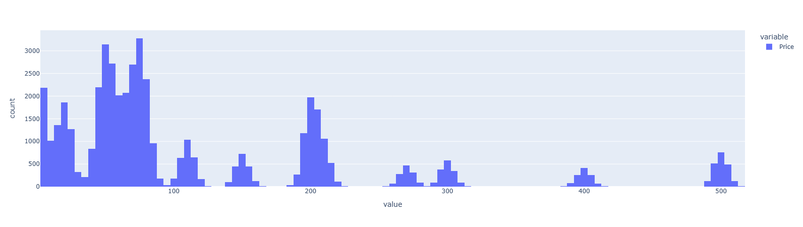
接下来创建并且拟合这个LinearRegression模型, 只有一点要注意, 就是这个X_train要从原始的DataFrame里面拿出列, 去to_numpy()然后再stack, Y_train因为那个price列每行只有一个数, 所以只要to_numpy()就好了
# TODO: Fit a linear regression model (price_model) on the training data with prices as the target variable
if (load_saved_models or IS_GRADING_ENV) and os.path.exists('price_model.joblib'):
    price_model = joblib.load('price_model.joblib')
    print("Model loaded from price_model.joblib")
else:
    price_model = LinearRegression()
    X_train=np.stack(prices_train['image'].to_numpy())
    Y_train=prices_train['Price'].to_numpy()
    price_model.fit(X=X_train, y=Y_train)

# TODO: Predict the prices of the test data and add them to the test_df
X_test=np.stack(prices_test['image'].to_numpy())再调用model.predict()得到测试结果, 加到测试集的DataFrame上去
prices_test['price_prediction'] = price_model.predict(X_test)

if save_models:
    joblib.dump(price_model, 'price_model.joblib')
print("Model saved to price_model.joblib")Problem 5b#
用numpy操作生成各种模型指标来评价模型在测试集上的表现, 要注意这里的变量基本上都是向量, 所以要想明白怎么用向量化操作
先看RMSE的计算
def compute_rmse(y_true, y_pred):
  length=len(y_true)
  rmse=np.sqrt(np.sum((y_true-y_pred)**2)/length)

return rmse向量的平方操作与除以标量是广播到每个分量上的, 最后的np.sum操作是对分量的聚合, 然后开根号
同理是MAE和R&2的计算
def compute_mae(y_true, y_pred):
  length=len(y_true)
  mae=np.sum(np.abs(y_true-y_pred))/length

  return mae


def compute_r2(y_true, y_pred):
  """Compute R-squared score"""
  R_Square=1-np.sum((y_true-y_pred)**2)/np.sum((y_true-np.mean(y_true))**2)

  return R_Square

def print_metrics(y_true, y_pred, dataset=""):
  """Print all regression metrics for a dataset"""
  rmse = compute_rmse(y_true, y_pred)
  mae = compute_mae(y_true, y_pred)
  r2 = compute_r2(y_true, y_pred)

  print(f"=== {dataset} Metrics ===")
  print(f"RMSE: {rmse:.2f}")
  print(f"MAE: {mae:.2f}")
  print(f"R²: {r2:.3f}")
return rmse, mae, r2顺便解释一下, 我感觉不像MSE和RMSE那么直观
当
的时候, 说明预测值和真实值完全一致
当
的时候, 说明统计意义下预测的方式和均值预测一样
当介于0到1且慢慢增大的时候, 就说明(总的)预测值和真实值是越来越靠近的
后面就是垃圾时间, 用model.predict得到预测值, 计算一些指标并且打印, 然后画个图就行了
# Calculate predictions
y_train_pred = price_model.predict(X_train_sc)
y_test_pred = price_model.predict(X_test_sc)

# Compute and print metrics
train_rmse, train_mae, train_r2 = print_metrics(prices_train['Price'], y_train_pred, "Training")
test_rmse, test_mae, test_r2 = print_metrics(prices_test['Price'], y_test_pred, "Test")

# Visualize predictions vs actual
fig = px.scatter(
    x=prices_test['Price'],
    y=y_test_pred,
    title='Predicted vs Actual Prices',
    labels={'x': 'Actual Price', 'y': 'Predicted Price'}
)
fig.add_trace(px.line(x=[prices_test['Price'].min(), prices_test['Price'].max()],
                      y=[prices_test['Price'].min(), prices_test['Price'].max()]).data[0])
fig.show()=== Training Metrics ===
RMSE: 118.72
MAE: 90.26
R²: -0.006
=== Test Metrics ===
RMSE: 121.58
MAE: 90.56
R²: -0.054数据上可以看出这个预测效果很差, 甚至不如均值预测
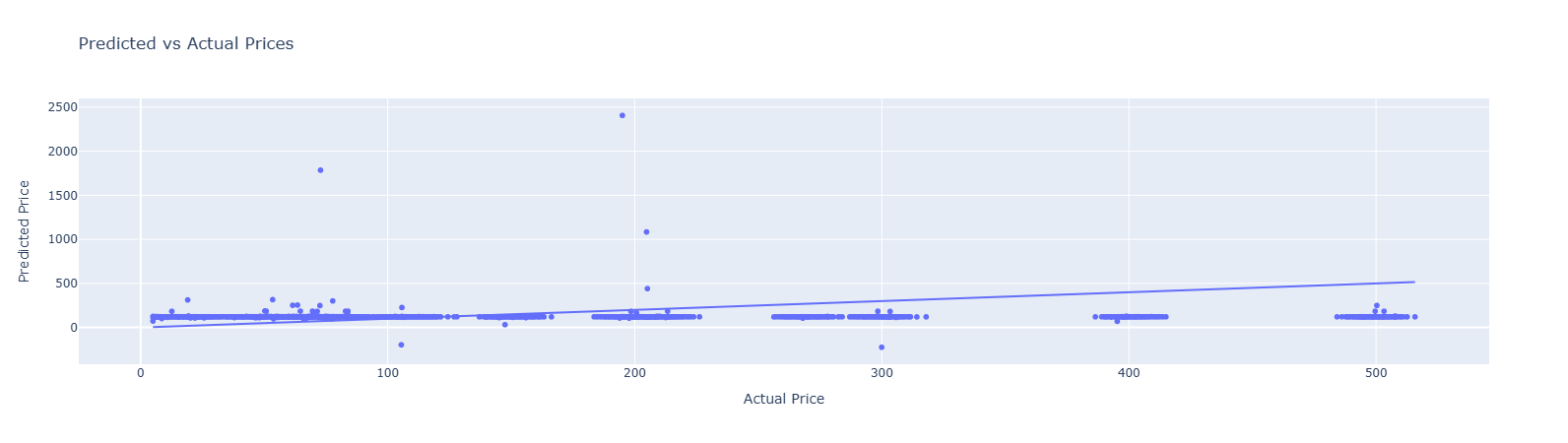
图上更直观, 可以看到大部分预测点当中, Predicted Price都被远远低估了, 距离那根
非常远, 和的结果一致
Problem 5d#
分类错误和回归误差
之前我们是对这份数据做了分类的, 即用那个2层的MLP分类器去预测label, 现在我们要研究一下分类对/错的类和回归的价格误差之间的一些关系
先看一下经过分类/回归之后已有的数据:
prices_test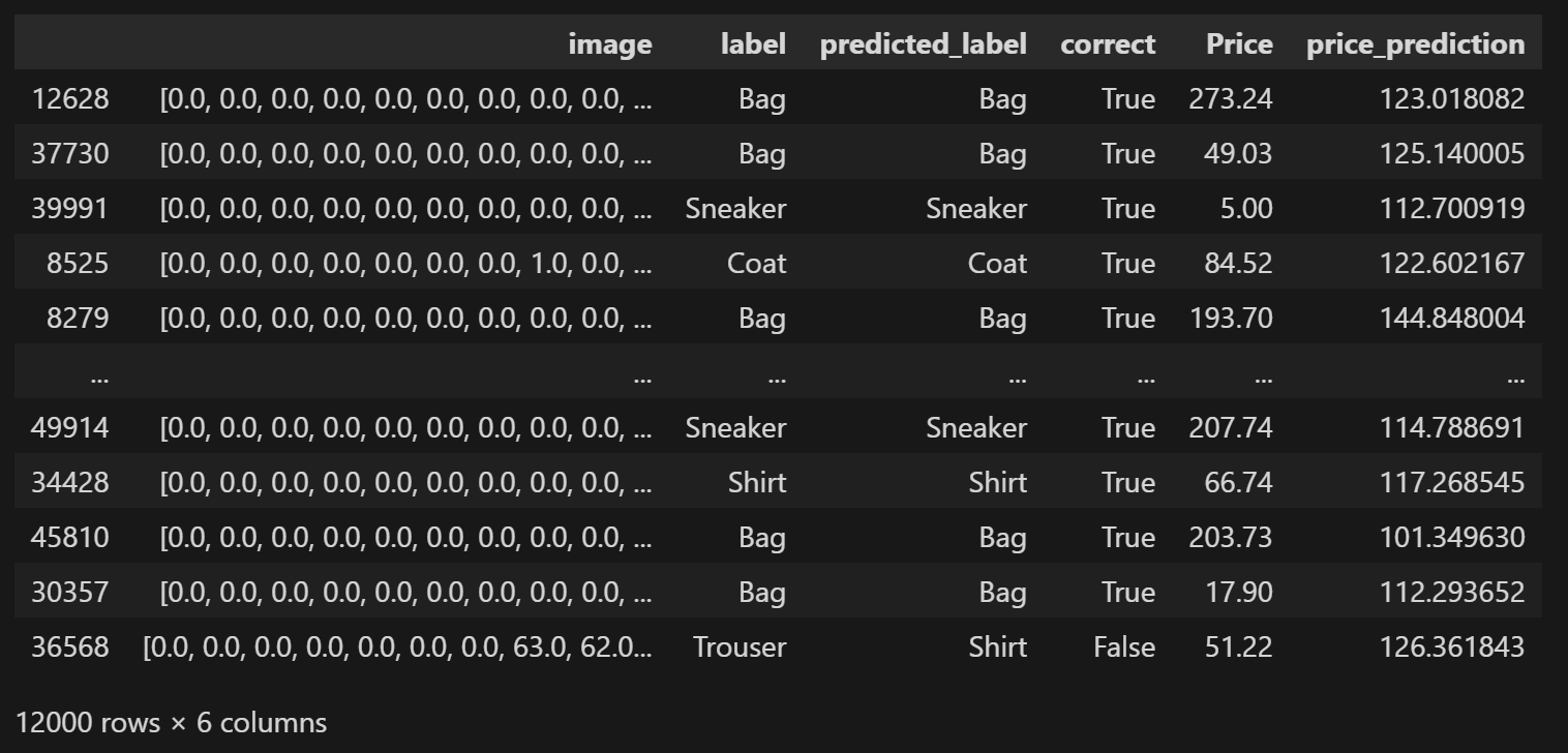
先计算两个误差: price_prediction和Price的差值的绝对值以及差值绝对值与真实值的商
# TODO: Compare how accurate the model is at classifying the images vs how accurate it is at predicting the price of the images
# TODO: Calculate the average relative price error for correctly classified vs. misclassified images
prices_test['price_error']=np.abs(prices_test['price_prediction']-prices_test['Price'])
prices_test['price_error_relative']=prices_test['price_error']/prices_test['Price']然后按预测label是否正确来分类, 在类内计算商误差的平均值, 这一步是为了看看分类对/错和回归误差之间有没有什么关系, 一个naive的想法是那些错误分类的点的回归误差的平均值应该要高一些
misclassified_price_error = prices_test[prices_test['correct']==False]['price_error_relative'].mean()
correctly_classified_price_error = prices_test[prices_test['correct']==True]['price_error_relative'].mean()


print(f"\nPrice prediction performance:")
print(f"Misclassified images - Avg relative price error: {misclassified_price_error:.3f}")
print(f"Correctly classified images - Avg relative price error: {correctly_classified_price_error:.3f}")Price prediction performance:
Misclassified images - Avg relative price error: 2.585
Correctly classified images - Avg relative price error: 2.321实际上只有非常小的差别
Problem 6a#
我们将在一个新的数据集上应用我们训练好的model(2层MLP分类器), 首先要对新数据集的数据(both训练集和测试集)做标准化
X_test_secret = np.load("./data/secret_test_set/X_test.npy")
y_test_secret = np.load("./data/secret_test_set/y_test.npy")

X_test_secret_sc = scaler.transform(X_test_secret)

print(X_test_secret.shape)
print(y_test_secret.shape)不记得了可以去前面看一下, 这个scaler变量是StandardScaler的实例, 他会自动学习均值和方差以便归一化
(2000, 784)
(2000,)接下来就是先把X和y装填进一个DataFrame里面, 然后调用model.predict得到预测值, 最后计算一些指标并且打印
# TODO: Create a dataframe with the secret test set and use the model to predict the labels
test_secret_df = pd.DataFrame()
test_secret_df['label'] = y_test_secret

test_secret_df['image'] = X_test_secret.tolist()
# test_secret_df['image'] = test_secret_df['image'].apply(lambda x: np.array(x).reshape(-1))

# TODO: Use the model to predict the labels and calculate the accuracy
test_secret_df['predicted_label'] = model.predict(X_test_secret_sc)

test_secret_df['correct'] = test_secret_df['predicted_label'] == test_secret_df['label']

print(f"Test accuracy: {test_df['correct'].mean():.3f}")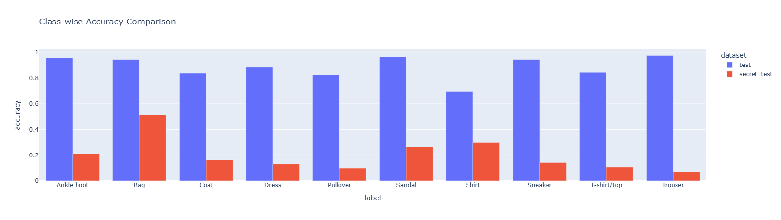
print(f"Secret Test accuracy: {test_secret_df['correct'].mean():.3f}")Test accuracy: 0.886
Secret Test accuracy: 0.200可以看到这个分类器在原来的测试集(其实应该叫验证集)上的正确率还可以, 但是真正在未知的测试集上的正确率非常低, 只有20%
Problem 6b#
在验证集/测试集上分label看正确率
test_df.groupby('label')['correct'].mean()label
Ankle boot 0.956775
Bag 0.943191
Coat 0.836106
Dress 0.882601
Pullover 0.824066
Sandal 0.963666
Shirt 0.692939
Sneaker 0.943054
T-shirt/top 0.842762
Trouser 0.974569
Name: correct, dtype: float64test_secret_df.groupby('label')['correct'].mean()label
Ankle boot 0.212963
Bag 0.513089
Coat 0.161290
Dress 0.130653
Pullover 0.098655
Sandal 0.265403
Shirt 0.297980
Sneaker 0.142857
T-shirt/top 0.107143
Trouser 0.070707
Name: correct, dtype: float64画个直方图
# TODO: Make a two-colored bar plot of the model's accuracy on the test set and the secret test set
result_df=pd.concat([test_df.groupby('label')['correct'].mean(),test_secret_df.groupby('label')['correct'].mean()],axis=1
,keys=['test','secret_test']).reset_index()

result_df_long = result_df.melt(
    id_vars='label',
    value_vars=['test', 'secret_test'],
    var_name='dataset',
    value_name='accuracy'
)

result_df_long.plot(
    x='label',
    y='accuracy',
    color='dataset',  # 按 dataset 列分组着色
    kind='bar',
    title='Class-wise Accuracy Comparison',
    barmode='group'  # 关键:设置为 'group' 实现分组显示
)
Problem 6c#
调用sklearn.confusion_matrix得到混淆矩阵
# TODO: plot a confusion matrix for the secret test set
y_true=test_secret_df['label']
y_pred=test_secret_df['predicted_label']
conf_matrix = confusion_matrix(y_true,y_pred)

conf_matrixarray([[ 46, 89, 2, 1, 7, 12, 17, 5, 27, 10],
[ 8, 98, 6, 3, 7, 17, 26, 2, 23, 1],
[ 1, 73, 30, 1, 13, 9, 47, 0, 10, 2],
[ 1, 49, 8, 26, 12, 28, 34, 13, 24, 4],
[ 1, 111, 13, 5, 22, 3, 53, 0, 11, 4],
[ 2, 27, 1, 7, 9, 56, 29, 14, 57, 9],
[ 0, 78, 9, 3, 13, 9, 59, 0, 25, 2],
[ 10, 21, 2, 12, 16, 33, 9, 30, 67, 10],
[ 1, 69, 2, 2, 18, 12, 45, 1, 18, 0],
[ 0, 24, 7, 23, 16, 51, 43, 8, 12, 14]])混淆矩阵表示真实label为, 预测label为的样本个数
Problem 6d#
首先利用给出的show_inages函数画出一些错误分类的例子
# Predict labels for the secret test set
predictions_secret = model.predict(X_test_secret_sc)

# Identify misclassified examples
incorrect_secret = predictions_secret != y_test_secret

# Generate labels for misclassified examples with true and predicted labels
labels = [f"True: {true_label}<br>Pred: {pred_label}"
          for true_label, pred_label in zip(y_test_secret[incorrect_secret], predictions_secret[incorrect_secret])]

# Display misclassified images with their true and predicted labels
show_images(X_test_secret[incorrect_secret], max_images=5, ncols=5, labels=labels, reshape=True)
图中可以看出测试集上所有的图片都旋转了, 也许因为这个导致分类器误判了(因为训练数据当中并没有旋转了的图片), 我们有以下三个方案来解决这个问题
- 把旋转了的图片加入训练集, 让模型学习额外的特征
- 把测试集的图片转回去, 重新预测
- Test Time Augmentation(TTA) 在测试时尝试多种增强图像的策略并且做出多个预测, 然后组合成最终的预测结果(和量化里的多路因子信号组合成最终信号差不多)
Problem 7a#
把训练数据当中的每一张图去rotate, 并记下旋转的角度, 得到一系列新的训练数据
def randomly_rotate_images(images, num_rotations_per_image=5):
  """
  Create training data by rotating original images and storing the rotation angles as labels.
  Params:
    - images: numpy array of shape (n_images, 784)
    - num_rotations_per_image: int, number of rotations to perform per image
  Returns:
    - X_augmented: numpy array of shape (n_images * num_rotations_per_image, 784)
    - y_rotations: numpy array of shape (n_images * num_rotations_per_image,)
  """
  # TODO: Implement this function

  X_augmented=[]
  y_rotations=[]

  for image in images:
    angles=np.random.uniform(low=0,high=360,size=num_rotations_per_image)

    image_2d=image.reshape(28,28)

    for angle in angles:
      rotated_2d=rotate(image_2d,angle,reshape=False,cval=0,order=1)

      rotated_1d=rotated_2d.flatten()

      X_augmented.append(rotated_1d)
      y_rotations.append(angle)


  return np.array(X_augmented),np.array(y_rotations)
  # raise NotImplementedError("Not implemented")

X_train = X_train[:3000]
y_train = y_train[:3000]

num_rotations_per_image = 4
X_train_rotated, y_train_rotations = randomly_rotate_images(X_train, num_rotations_per_image)
y_train_augmented = np.array([y for label in y_train for y in [label]*num_rotations_per_image])
# y_train_augmented = np.repeat(y_train, num_rotations_per_image)
print(X_train_rotated.shape)
print(y_train_augmented.shape)

show_images(X_train_rotated, max_images=5, ncols=5, labels=y_train_augmented, reshape=True)记得要flatten一下就好

Problem 7b#
用新得到的训练数据去训练一个新的模型, 注意标签还是和原来一样的, 因为数据旋转并不改变label
X_train_rotated_sc = scaler.transform(X_train_rotated)
X_test_secret_sc = scaler.transform(X_test_secret)

if load_saved_models:
  model_rotated = joblib.load('mlp_fashionmnist_rotated_model.joblib')
else:
  # TODO: initialize and train a new model on the rotated images
  model_rotated =  MLPClassifier()
  model_rotated.fit(X=np.stack(X_train_rotated_sc),y=y_train_augmented)

  if save_models:
    joblib.dump(model_rotated, "mlp_fashionmnist_rotated_model.joblib")
    print("Rotated model saved to disk.")

print(f"Training accuracy (training on rotated images): {model_rotated.score(X_train_rotated_sc, y_train_augmented):.3f}")
print(f"Test accuracy (original): {model.score(X_test_sc, y_test):.3f}")
print(f"Test accuracy (training on rotated images): {model_rotated.score(X_test_secret_sc, y_test_secret):.3f}")

loss_df = pd.DataFrame({
    'epoch': range(1, len(model_rotated.loss_curve_) + 1),
    'loss': model_rotated.loss_curve_
})
loss_df.plot(x='epoch', y='loss', title="Training Error")Rotated model saved to disk.
Training accuracy (training on rotated images): 1.000
Test accuracy (original): 0.886
Test accuracy (training on rotated images): 0.689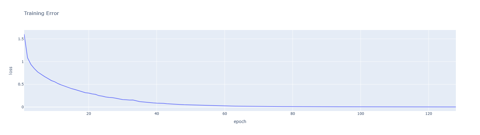
Problem 8a#
这个问题逻辑比较复杂, 首先我们刚刚得到了一些旋转的数据, 也就是(图片, 旋转角度), 我们可以用这些数据去训练一个简单的神经网络回归模型(MLPRegressor), 让他学习根据图片的状态预测旋转的角度, 然后在把测试集图片输入这个模型去得到测试集的旋转角度, 这样就可以逆向旋转回来了
训练阶段:
┌────────────────┐     ┌────────────────┐     ┌────────────────────┐
│  图片 + 角度    │ ──→ │  MLPRegressor  │ ──→ │  模型学会预测角度   │
│  (有标签的)     │     │  回归模型       │     │  image → rotation  │
└────────────────┘     └────────────────┘     └────────────────────┘

预测阶段:
┌────────────────┐     ┌────────────────┐     ┌────────────────────┐
│  测试集图片     │ ──→ │  预测旋转角度   │ ──→ │  逆时针转回来      │
│  (被旋转过的)   │     │  比如 30°      │     │  30° → 0°         │
└────────────────┘ └────────────────┘ └────────────────────┘if (load_saved_models or IS_GRADING_ENV) and os.path.exists('model_rotation_regression.joblib'):
model_rotation_regression = joblib.load("model_rotation_regression.joblib")
else:
# Train a larger regression model (MLP) to predict rotation angles
model_rotation_regression = MLPRegressor(
hidden_layer_sizes=(256, 128),
activation='relu',
solver='adam',
max_iter=100,
random_state=SEED,
early_stopping=True,
verbose=True
)
# TODO: train a MLP regressor to predict rotation angles
model_rotation_regression.fit(X=X_train_rotated_sc,y=y_train_rotations)
# Save model_rotation_regression and scaler
if save_models:
joblib.dump(model_rotation_regression, "model_rotation_regression.joblib")
joblib.dump(scaler, "scaler.joblib")
print("Rotation regression model and scaler saved to disk.")
loss_df = pd.DataFrame({
'epoch': range(1, len(model_rotation_regression.loss_curve_) + 1),
'loss': model_rotation_regression.loss_curve_
})
loss_df.plot(x='epoch', y='loss', title="Training Loss")迭代一百次就够了, 只是一个简单的神经网络而已
Iteration 1, loss = 9611.26410087
Validation score: 0.142763
Iteration 2, loss = 3766.69187363
Validation score: 0.385691
Iteration 3, loss = 2920.89570158
Validation score: 0.484820
Iteration 4, loss = 2530.66131818
Validation score: 0.523250
Iteration 5, loss = 2275.49896874
Validation score: 0.559317
Iteration 6, loss = 2085.74463183
Validation score: 0.584974
Iteration 7, loss = 1924.98972761
Validation score: 0.602003
Iteration 8, loss = 1804.65769176
Validation score: 0.618211
Iteration 9, loss = 1682.16687650
Validation score: 0.631943
Iteration 10, loss = 1571.02563443
Validation score: 0.640702
Iteration 11, loss = 1478.80508676
Validation score: 0.653446
Iteration 12, loss = 1392.98262424
Validation score: 0.655017
Iteration 13, loss = 1316.21452457
Validation score: 0.674004
Iteration 14, loss = 1236.47938882
Validation score: 0.679636
Iteration 15, loss = 1161.99735384
Validation score: 0.687010
Iteration 16, loss = 1105.28316375
Validation score: 0.699418
Iteration 17, loss = 1048.20584135
Validation score: 0.693873
Iteration 18, loss = 977.81792593
Validation score: 0.711631
Iteration 19, loss = 925.44572624
Validation score: 0.699191
Iteration 20, loss = 899.88230979
Validation score: 0.702843
Iteration 21, loss = 840.36804019
Validation score: 0.729254
Iteration 22, loss = 780.98734272
Validation score: 0.728786
Iteration 23, loss = 765.77998552
Validation score: 0.734939
Iteration 24, loss = 705.92240284
Validation score: 0.737799
Iteration 25, loss = 674.86031295
Validation score: 0.735162
Iteration 26, loss = 634.87954343
Validation score: 0.745473
Iteration 27, loss = 589.66117117
Validation score: 0.745895
Iteration 28, loss = 579.90028943
Validation score: 0.744533
Iteration 29, loss = 543.20496845
Validation score: 0.734867
Iteration 30, loss = 505.46502073
Validation score: 0.747184
Iteration 31, loss = 475.18828419
Validation score: 0.750737
Iteration 32, loss = 451.34752457
Validation score: 0.752262
Iteration 33, loss = 432.74789467
Validation score: 0.735379
Iteration 34, loss = 403.09219879
Validation score: 0.756212
Iteration 35, loss = 375.65089303
Validation score: 0.752666
Iteration 36, loss = 356.99911305
Validation score: 0.763152
Iteration 37, loss = 333.24136299
Validation score: 0.755819
Iteration 38, loss = 317.56468084
Validation score: 0.763254
Iteration 39, loss = 300.31424482
Validation score: 0.752810
Iteration 40, loss = 292.59236521
Validation score: 0.763904
Iteration 41, loss = 283.44042869
Validation score: 0.748904
Iteration 42, loss = 274.85827460
Validation score: 0.762908
Iteration 43, loss = 242.64105699
Validation score: 0.762618
Iteration 44, loss = 224.33508193
Validation score: 0.755256
Iteration 45, loss = 209.78245760
Validation score: 0.764000
Iteration 46, loss = 198.72396655
Validation score: 0.760627
Iteration 47, loss = 195.43882927
Validation score: 0.752333
Iteration 48, loss = 184.33454222
Validation score: 0.762145
Iteration 49, loss = 176.41046927
Validation score: 0.762408
Iteration 50, loss = 165.02544010
Validation score: 0.752812
Iteration 51, loss = 165.35008826
Validation score: 0.752220
Validation score did not improve more than tol=0.000100 for 10 consecutive epochs. Stopping.
Rotation regression model and scaler saved to disk.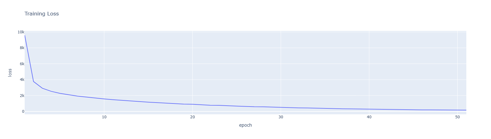
Problem 8b#
现在来检测一下这个角度回归模型的效果
利用X_test这个数据集, 先把他旋转并且记下旋转的角度y_test_rotations, 然后用角度回归模型来预测这个旋转角度, 和y_test_rotations计算MSE和RMSE就知道模型的效果了
# TODO: Use the model_rotation_regression to predict the rotation angles on X_test_rotated_sc
X_test_rotated, y_test_rotations = randomly_rotate_images(X_test,num_rotations_per_image=1)
X_test_rotated_sc = scaler.transform(X_test_rotated)

y_pred_angles = model_rotation_regression.predict(X_test_rotated_sc)
mse = mean_squared_error(y_test_rotations,y_pred_angles)
rmse = np.sqrt(mse)
print(f"Test MSE: {mse:.2f}")
print(f"Test RMSE: {rmse:.2f} degrees")

# Show some predictions
print("\nSample predictions:")
for i in range(5):
    print(f"True rotation: {y_test_rotations[i]:.1f}°, Predicted: {y_pred_angles[i]:.1f}°")

print("------------------------------")
print("------------------------------")
print(f"Test MSE (angle):  {mse:.2f}")
print(f"Test RMSE:        {rmse:.2f}°")
print("------------------------------")
print("------------------------------")Test MSE: 3748.14
Test RMSE: 61.22 degrees
Sample predictions:
True rotation: 263.5°, Predicted: 196.7°
True rotation: 188.1°, Predicted: 154.8°
True rotation: 32.8°, Predicted: 32.1°
True rotation: 337.8°, Predicted: 330.9°
True rotation: 295.0°, Predicted: 328.0°
------------------------------
------------------------------
Test MSE (angle): 3748.14
Test RMSE: 61.22°
------------------------------
------------------------------Plot出来
# Create scatter plot of predictions vs actual
scatter_fig = go.Figure()
scatter_fig.add_trace(
    go.Scatter(
        x=y_test_rotations[:200],  # First 200 samples for clarity
        y=y_pred_angles[:200],
        mode='markers',
        name='Predictions',
        marker=dict(size=6, opacity=0.7)
    )
)

# Add perfect prediction line
max_angle = max(y_test_rotations[:200])
scatter_fig.add_trace(
    go.Scatter(
        x=[0, max_angle],
        y=[0, max_angle],
        mode='lines',
        name='Perfect Prediction',
        line=dict(dash='dash', color='red')
    )
)

scatter_fig.update_layout(
    title='Predicted vs Actual Rotation Angles',
    xaxis_title='Actual Angle (degrees)',
    yaxis_title='Predicted Angle (degrees)',
    width=600,
    height=500
)

scatter_fig.show()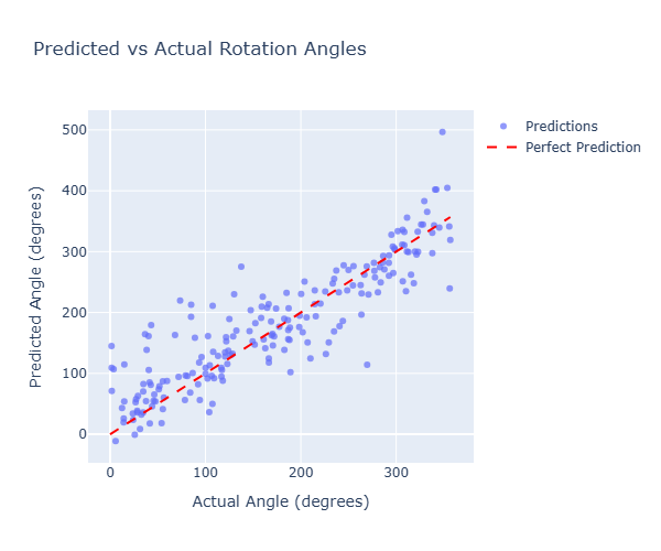
可以看到预测的效果还是不错的
画个例子, 输出原始图像, 旋转后的图像, 以及根据角度模型输出逆向旋转后的图像
# Demonstrate unrotation using predicted angles
def unrotate_image(rotated_image, predicted_angle):
    """
    Unrotate an image by rotating it by the negative of the predicted angle.
    """
    return rotate_image_by_angle(rotated_image, -predicted_angle)

# Test unrotation on a sample
sample_idx = 0
original_test_image = X_test[sample_idx // 1]  # Get original unrotated image
rotated_test_image = X_test_rotated[sample_idx] # Get the rotated image
true_angle = y_test_rotations[sample_idx] # Get the true angle the image was rotated by
predicted_angle = y_pred_angles[sample_idx] # Get the model's prediction
unrotated_image = unrotate_image(rotated_test_image, predicted_angle)

# Prepare images and titles for display
images = [
    original_test_image.reshape(28, 28)[::-1],
    rotated_test_image.reshape(28, 28)[::-1],
    unrotated_image.reshape(28, 28)[::-1]
]
titles = [
    'Original',
    f'Rotated by {true_angle:.1f}°',
    f'After unrotating the image with the model\'s prediction (pred: {predicted_angle:.1f}°)'
]

# Create a subplot grid using plotly express imshow
fig = px.imshow(
    np.stack(images),
    facet_col=0,
    facet_col_wrap=3,
    color_continuous_scale='gray',
    aspect='auto'
)

# Update facet titles
for i, title in enumerate(titles):
    fig.layout.annotations[i]['text'] = title

fig.update_layout(
    height=300,
    width=1200,
    title_text="Image Rotation Prediction and Correction",
    coloraxis_showscale=False
)
fig.update_xaxes(showticklabels=False, showgrid=False, zeroline=False)
fig.update_yaxes(showticklabels=False, showgrid=False, zeroline=False)
fig.show()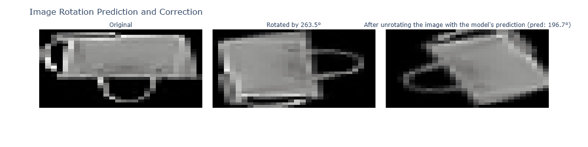
Problem 8c#
先预测一下测试集旋转的角度, 再逆向旋转
# TODO: Scale the secret test set and use model_rotation_regression to unrotate the images in the secret test set
X_test_secret_scaled = scaler.transform(X_test_secret)
y_pred_angles = model_rotation_regression.predict(X_test_secret_scaled)
X_test_unrotated  = np.array([
    rotate_image_by_angle(X_test_secret[i],-y_pred_angles[i])
    for i in range(len(X_test_secret))
])
X_test_unrotated_sc = scaler.transform(X_test_unrotated)接着对这个逆向旋转的数据去预测label, 注意这个逆向旋转之后的图和之前的是一一对应的, 本质上还是在预测之前的label, 逆向旋转只是个增强而已
# TODO: Make new predictions using the original MLPClassifier model and check which images are correctly classified
test_secret_df["unrotated_prediction"] = model.predict(X_test_unrotated)
test_secret_df["unrotated_correct"] = test_secret_df["unrotated_prediction"] == test_secret_df['label']

print(f"Test accuracy: {test_secret_df.correct.mean():.3f}")
print(f"Unrotated Test accuracy: {test_secret_df.unrotated_correct.mean():.3f}")Test accuracy: 0.200
Unrotated Test accuracy: 0.243可以看到有增强
接下来我们对比一下这三种方式的绩效
-原始baseline(直接跑测试集) -先用旋转过的数据去训练模型, 然后再跑测试集合 -训练角度预测模型, 把原数据逆向旋转之后再跑
# Compare all three approaches
baseline_accuracy = model.score(X_test_secret_sc, y_test_secret) # method: baseline
rotated_training_accuracy = model_rotated.score(X_test_secret_sc, y_test_secret) # method: train on rotated images
unrotated_accuracy = model.score(X_test_unrotated_sc, y_test_secret) # method: predict & unrotate, then classify the images we tried to unrotate

# Create comparison DataFrame
comparison_df = pd.DataFrame({
    'Method': ['Baseline (no handling)', 'Train on rotated images', 'Predict & unrotate'],
    'Accuracy': [baseline_accuracy, rotated_training_accuracy, unrotated_accuracy]
})

# Plot comparison
fig = px.bar(
    comparison_df,
    x='Method',
    y='Accuracy',
    title='Comparison of Rotation Handling Methods',
    color='Accuracy',
    color_continuous_scale='RdYlGn'
)
fig.update_layout(
    xaxis_title="Method",
    yaxis_title="Test Accuracy",
    yaxis=dict(range=[0, 1])
)
fig.show()

print("\n=== Summary of All Methods ===")
for _, row in comparison_df.iterrows():
print(f"{row['Method']}: {row['Accuracy']:.3f}")Problem 9#
利用TTA的方式, 把每一个图像增强(旋转)得到很多个, 然后对他们预测取一个平均的概率得到结果
┌─────────────────────────────────────────────────────────────────┐
│                      test_time_augmentation 函数                │
├─────────────────────────────────────────────────────────────────┤
│                                                                 │
│   输入: image (原始测试图片)                                     │
│                                                                 │
│   Step 1: 预处理                                                 │
│   ┌─────────────────────────────────────────────────────────┐  │
│   │ image → 展平 → 标准化                                    │  │
│   └─────────────────────────────────────────────────────────┘  │
│                          │                                      │
│                          ▼                                      │
│   Step 2: 预测旋转角度并纠正                                     │
│   ┌─────────────────────────────────────────────────────────┐  │
│   │ model_rotation_regressor.predict() → 预测角度           │  │
│   │ rotate_image_by_angle(..., -angle) → 转回来            │  │
│   └─────────────────────────────────────────────────────────┘  │
│                          │                                      │
│                          ▼                                      │
│   Step 3: 多角度 TTA 预测                                       │
│   ┌─────────────────────────────────────────────────────────┐  │
│   │ 对 unrotated 图像应用 9 种角度旋转:                     │  │
│   │ -20°, -15°, -10°, -5°, 0°, 5°, 10°, 15°, 20°          │  │
│   │ 对每种旋转后的图像 → 标准化 → model.predict_proba()     │  │
│   │ 收集所有概率向量                                          │  │
│   └─────────────────────────────────────────────────────────┘  │
│                          │                                      │
│                          ▼                                      │
│   Step 4: 额外预测                                               │
│   ┌─────────────────────────────────────────────────────────┐  │
│   │ 原始图像的预测 + 转回来图像的预测                        │  │
│   └─────────────────────────────────────────────────────────┘  │
│                          │                                      │
│                          ▼                                      │
│   Step 5: 聚合与最终预测                                         │
│   ┌─────────────────────────────────────────────────────────┐  │
│   │ avg_probs = mean(all_probs)  # 11个概率向量取平均       │  │
│   │ prediction = argmax(avg_probs)  # 选择概率最大的类      │  │
│   └─────────────────────────────────────────────────────────┘  │
│                                                                 │
│   输出: class_dict[prediction]  # 返回类别标签                   │
└─────────────────────────────────────────────────────────────────┘代码看起来很长, 但其实都是流水线, 核心就是一张图片变多张图片, 产生多个概率向量, 求平均在argmax即可
# TODO: Write a function (or functions!) that can be used to improve the accuracy of the original MLPClassifer model using test time augmentations
# Feel free to add additional functions, arguments, etc. as needed!
def test_time_augmentation(model, scaler, image):
    """
    Predict a label using test-time augmentation
    Params:
        - model: the MLPClassifier model
        - scaler: the StandardScaler used to scale the images
        - image: the image to be augmented
    Returns:
        - prediction: the predicted label
    """
    ...
    # raise NotImplementedError("Not implemented")
    image = np.array(image, dtype=np.float64).reshape(-1)
    image_scaled=scaler.transform([image])
    predicted_angle=model_rotation_regression.predict(image_scaled)[0]

    unrotated=rotate_image_by_angle(image,-predicted_angle)

    test_angles=[-20,-15,-10,-5,0,5,10,15,20]

    all_probs=[]

    for angle in test_angles:
        rotated=rotate_image_by_angle(unrotated,angle)
        rotated_scaled=scaler.transform([rotated])
        probs=model.predict_proba(rotated_scaled)[0]
        all_probs.append(probs)

    original_scaled=scaler.transform([image])
    unrotated_scaled=scaler.transform([unrotated])
    all_probs.append(model.predict_proba(original_scaled)[0])
    all_probs.append(model.predict_proba(unrotated_scaled)[0])

    avg_probs=np.mean(all_probs,axis=0)
    prediction=np.argmax(avg_probs)

    return class_dict[prediction]


# Make a copy of the test secret dataframe and apply the test time augmentation to the images to get new predictions!
part_2_df = test_secret_df.copy()
part_2_df["image"] = part_2_df["image"].apply(lambda x: np.array(x).reshape(-1))
part_2_df["prediction"] = part_2_df["image"].apply(lambda x: test_time_augmentation(model_rotated, scaler, x))

# Check the accuracy of the new predictions
correct = part_2_df["prediction"] == part_2_df["label"]
print("Accuracy:", correct.mean())Accuracy: 0.341