CS189 Assignment1#
189这门课感觉也是理论和实践并行教学, Written Part的作业也不少, 不过比起336那种工程性质极强的课程来说还是容易不少, 至少这第一个Assignment没有和336那样, 一上来就整一大堆手搓, 189的作业基本上就是理解原来并调包, 极少的自己实现, 非常适合有志于成为API工程师的人学习
Written Part的数学作业也并不容易, 后面有机会写一些Notes
作业要求#
基本上是Fill in the Blanks性质的Lab, 把函数里面的所有TODO填满就行了, 几乎不需要自己设计接口
评测框架#
用的是UC Berkeley自行设计的otter框架, 一键安装就行了:
pip install otter-grader环境配置#
每个hw文件当中都给了requirements.txt, 直接安装就行
pip install -r requirements.txt除此之外就是配置一下网络环境, 由于我是在GPU服务器上运行的, 所以一些没找到镜像站的数据下载代码我就用反向ssh端口让他走我本地的代理, 打开本地终端开启这个反向ssh:
(base) liziyu@liziyudeMacBook-Pro ~ % ssh -R 7891:localhost:7890 zyli@lab
Welcome to Ubuntu 24.04.3 LTS (GNU/Linux 6.14.0-29-generic x86_64)

 * Documentation:  https://help.ubuntu.com
 * Management:     https://landscape.canonical.com
 * Support:        https://ubuntu.com/pro

Expanded Security Maintenance for Applications is not enabled.

124 updates can be applied immediately.
To see these additional updates run: apt list --upgradable

Enable ESM Apps to receive additional future security updates.
See https://ubuntu.com/esm or run: sudo pro status

*** System restart required ***
Last login: Fri Jan 23 15:16:55 2026 from 61.169.135.222
(base) zyli@lab:~$ 然后在notebook里面通过os来配置一下端口:
import os
where="lab"
# where="local"

if where=="lab":

    os.environ['HTTP_PROXY'] = 'http://localhost:7891'
os.environ['HTTPS_PROXY'] = 'http://localhost:7891'这里其实是比较烦的, 我本人还是喜欢去运行py文件, 用ALL_PROXY=localhost:7891的形式去做
Assignment Overview#
第一部分的所有代码在fashion_pt_1.ipynb里面, 都是一些比较基础的pandas和numpy的操作, 还有一些画图之类的, 主要就是让学习者习惯数据预处理
加载Fashion-MNIST数据集#
搞清楚数据集本身作为一个对象有什么属性就行
# Load the FashionMNIST dataset from torchvision
train_data = torchvision.datasets.FashionMNIST(root='./data', train=True, download=True)

# Extract the image data and convert it to a numpy array of type float
images = train_data.data.numpy().astype(float)

# Extract the target labels as a numpy array
targets = train_data.targets.numpy()

# Create a dictionary mapping class indices to class names
class_dict = {i: class_name for i, class_name in enumerate(train_data.classes)}

# Map the target labels to their corresponding class names
labels = np.array([class_dict[t] for t in targets])

# Create a list of class names in order of their indices
class_names = [class_dict[i] for i in range(len(class_dict))]

# Get the total number of samples in the dataset
n = len(images)

# Ensure class_names is a list of class names (redundant but ensures consistency)
class_names = list(class_dict.values())

# Print dataset information for verification
print("Loaded FashionMNIST dataset with {} samples.".format(n))
print("Classes: {}".format(class_dict))
print("Image shape: {}".format(images[0].shape))  # Shape of a single image
print("Image dtype: {}".format(images[0].dtype))  # Data type of the image array
print("Image type: {}".format(type(images[0]))) # Type of the image objectLoaded FashionMNIST dataset with 60000 samples.
Classes: {0: 'T-shirt/top', 1: 'Trouser', 2: 'Pullover', 3: 'Dress', 4: 'Coat', 5: 'Sandal', 6: 'Shirt', 7: 'Sneaker', 8: 'Bag', 9: 'Ankle boot'}
Image shape: (28, 28)
Image dtype: float64
Image type: <class 'numpy.ndarray'>Problem 0a#
从数据集的两列numpy.series:images和targets构造DataFrame
# TODO: Create a DataFrame with two columns: `image` and `label`

...
image_list=images.tolist()
label_list=labels.tolist()

df=pd.DataFrame({'image':image_list,'label':label_list})
df['image']=df['image'].apply(np.array)

# Print the shape and columns of the DataFrame
print("DataFrame shape:", df.shape)
print("DataFrame columns:", df.columns.tolist())
df.head()DataFrame shape: (60000, 2)
DataFrame columns: ['image', 'label']
Problem 1a#
计算数据集每个label出现的个数, 然后看每个label出现的个数是否相等
# TODO: Calculate the distribution of labels using `value_counts()``
# TODO: Compare the min and max values of `label_distribution` to determine if the dataset is balanced.

label_distribution=df['label'].value_counts()
is_balanced=label_distribution.min()==label_distribution.max()

print(f"Label distribution:\n{label_distribution}")
print(f"Is the dataset balanced? {is_balanced}")Label distribution:
label
Ankle boot 6000
T-shirt/top 6000
Dress 6000
Pullover 6000
Sneaker 6000
Sandal 6000
Trouser 6000
Shirt 6000
Coat 6000
Bag 6000
Name: count, dtype: int64
Is the dataset balanced? TrueProblem 1b#
用groupby()分组并且统计每个组的行数
# TODO: Group the rows in `df` according to the values in the `labels` column. Then, count the number of rows in each group.
label_distribution_groupby = df.groupby('label').size()

label_distribution_groupbylabel
Ankle boot 6000
Bag 6000
Coat 6000
Dress 6000
Pullover 6000
Sandal 6000
Shirt 6000
Sneaker 6000
T-shirt/top 6000
Trouser 6000
dtype: int64Problem 1c#
对label列进行可视化
# Plotting library to use, default is matplotlib but plotly has more functionality
pd.options.plotting.backend = "plotly"

# TODO: Plot a histogram of the labels in the DataFrame `df` using the DataFrame's built-in plotting functions (this should be 1 line)
df['label'].plot(kind="hist")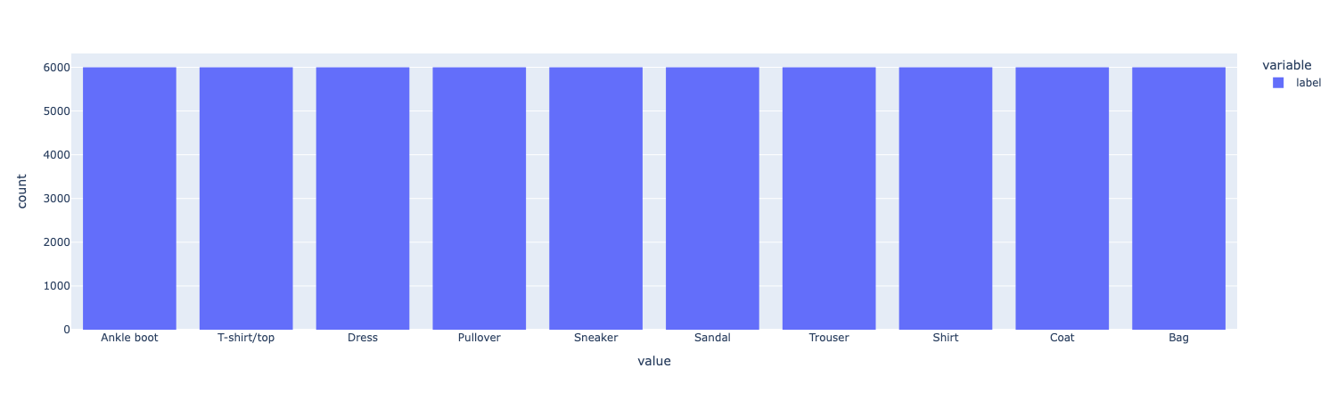
课程组还给了一个show_images函数, 他会打出图片和label
def show_images(images, max_images=40, ncols=5, labels = None, reshape=False):
    """Visualize a subset of images from the dataset.
    Args:
        images (np.ndarray or list): Array of images to visualize [img,row,col].
        max_images (int): Maximum number of images to display.
        ncols (int): Number of columns in the grid.
        labels (np.ndarray, optional): Labels for the images, used for facet titles.
    Returns:
        plotly.graph_objects.Figure: A Plotly figure object containing the images.
    """
    if isinstance(images, list):
        images = np.stack(images)
    n = min(images.shape[0], max_images) # Number of images to show
    px_height = 220 # Height of each image in pixels
    if reshape:
        images = images.reshape(images.shape[0], 28, 28)
    fig = px.imshow(images[:n, :, :], color_continuous_scale='gray_r',
                    facet_col = 0, facet_col_wrap=ncols,
                    height = px_height * int(np.ceil(n/ncols)))
    fig.update_layout(coloraxis_showscale=False)
    fig.update_xaxes(showticklabels=False, showgrid=False)
    fig.update_yaxes(showticklabels=False, showgrid=False)
    if labels is not None:
        # Extract the facet number and replace with the label.
        fig.for_each_annotation(lambda a: a.update(text=labels[int(a.text.split("=")[-1])]))
return fig后面会用到
Problem 1d#
用groupby分类, 然后在每个分类里面挑两张图, 打印出图和他的分类
# TODO: Get 2 sample images per class and plot them.
examples = df.groupby('label').head(2)

fig = show_images(examples["image"].tolist(), ncols=4, labels=examples["label"].tolist())
fig.show()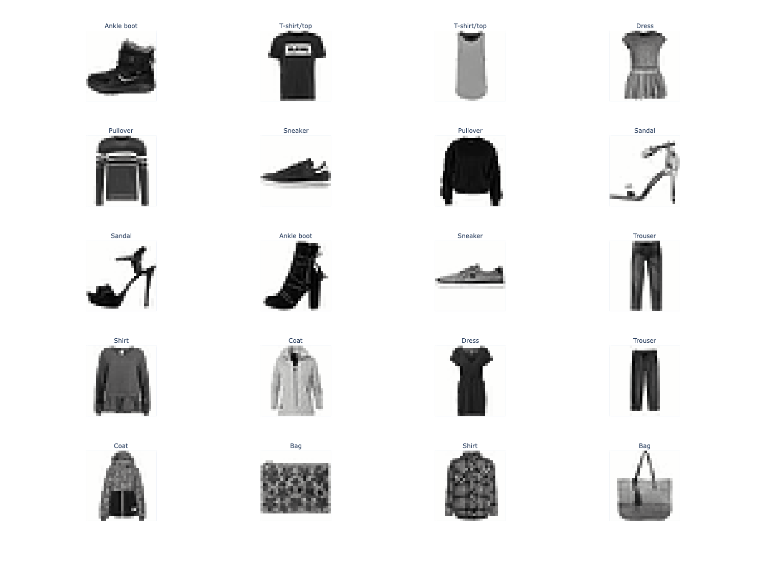
Problem 2#
用reshape函数把一个m*n的图像变成mn*1的
df["image"] = df["image"].apply(lambda img: img.reshape(-1))原始的每行的image元素都是28*28的, 现在每行都变成784*1的了
np.stack(df['image'].values).shape(60000, 784)这里说一下这个np.stack(arrays, axis, out)的用法, 以前每次都是AI写, 不太清楚其中原理
np.stack作用于一些数组, 这些数组必须有相同的shape, 沿着axis指定的轴拼起来, 这会加入第n+1个维度, 就像两本书叠起来, 显然要有一个z轴来标识这是第一本书还是第二本书
a = np.array([1, 2, 3])
b = np.array([4, 5, 6])
np.stack((a, b))
# array([[1, 2, 3],
#        [4, 5, 6]]) 2*3, 第0维出现一个2

np.stack((a, b), axis=-1)
# array([[1, 4],
#        [2, 5],
# [3, 6]]) 3*2, 第1维出现一个3简而言之就是axis是多少, 结果在第axis个维度上就会出现一个n, n是数组的个数
Problem 2a#
调用sklearn.KMeans进行聚类
# TODO: Perform k-means clustering on the images (10 clusters to match the number of classes)
from sklearn.cluster import KMeans

df_sample = df.sample(n=1000, random_state=SEED)
kmeans=KMeans(n_clusters=10,random_state=SEED)
X=np.stack(df_sample['image'].to_numpy())
cluster_labels=kmeans.fit_predict(X)

kmeans_df=df_sample.assign(cluster=cluster_labels)

kmeans_df.head(3)这里的np.stack就是把一堆图片点聚集起来, 现在这个kmeans_df有了一个新的列cluster, 代表聚类的结果, 比如说会把一些行聚类成1类, 2类…以此类推, 总共10个类
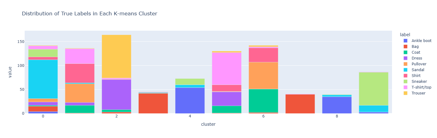
Problem 2b#
评估KMeans聚类的效果
只需要对label(聚类的结果)groupby一下然后看每个聚类里面有多少种不同的true_label, 如果聚类的效果比较好的话, 应该每种聚类里面有尽可能少的true_label种类
# TODO: Create a stacked bar plot of the label counts per cluster.
cluster_label_counts = kmeans_df.groupby(['cluster', 'label']).size().unstack(fill_value=0)

cluster_label_counts.plot(
    kind='bar',
    title='Distribution of True Labels in Each K-means Cluster'
)
上面的数据操作有点烦人, 一不小心就会写错, 这其实是一个类似于pivot的操作, 经过groupby([“cluster”,“label”]).size()之后会有一个二级索引
    cluster  label
    0        0         50
             1         12
             2         5
    1        0         10
             2         80
...unstack之后会把内层索引index变成列名, 这就创建了(cluster,label)到count的一一映射, 然后就可以画图了
cluster  label0  label1  label2
0        50      12      5
1        10      80      0
...这样一来count就成了没名字的元素了
Problem 2c#
在每个Cluster里面随机抽出7个图片, 把他们打出来
# TODO: Plot 7 images from each cluster (use the show_images function, 10 rows, 7 columns)
Cluster_Head=kmeans_df.groupby('cluster').sample(n=7,random_state=SEED)

fig = show_images(Cluster_Head["image"].tolist(), ncols=7, labels=Cluster_Head["cluster"].tolist(),reshape=True,max_images=70)
fig.show()

# Cluster_Head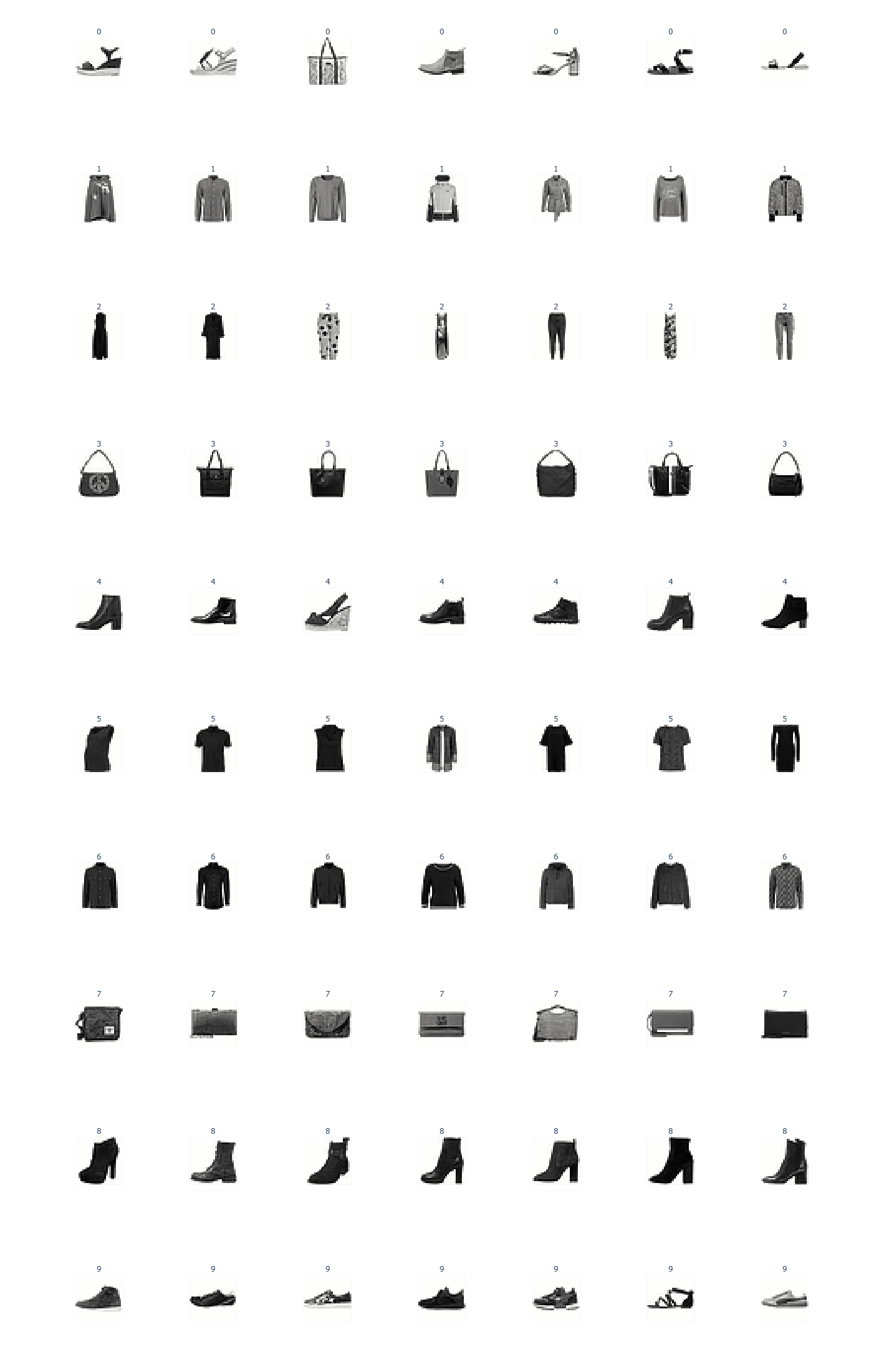
可以看到聚类的效果还是不错的, 至少没把衣服和鞋子放一起去
Problem 3#
训练一个MLP分类器, 总共四个步骤
数据预处理模型训练绩效评估可视化
先进行训练集和测试集的切分, 不能用train_test_split, 其实也很简单, 先sample出训练集, 那不在训练集里面的就是测试集
df_copy = df.copy()
train_df = df_copy.groupby('label').sample(frac=0.8, random_state=SEED)
test_df = df_copy[~df_copy.index.isin(train_df.index)]
print(f"Training set size: {len(train_df)}")
print(f"Test set size: {len(test_df)}")Problem 3a#
展平并归一化数据点, 启动训练并且绘制损失曲线
# flatten features into 1D arrays
X_train = np.stack(train_df['image'].values)
y_train = train_df['label'].values
X_test = np.stack(test_df['image'].values)
y_test = test_df['label'].values

print(f"X_train shape: {X_train.shape}\t y_train shape: {y_train.shape}")
print(f"X_test shape: {X_test.shape}\t y_test shape: {y_test.shape}")

# TODO: Train the model using the scaled traning data and plott the loss curve (remeber to normalize your data!)
# NOTE: Your model must be named `model`
def flatten(images):
    return images.reshape(images.shape[0], -1)
image_scalar=StandardScaler()
image_scalar.fit(flatten(X_train))
X_train_sc=image_scalar.transform(flatten(X_train))
X_test_sc=image_scalar.transform(flatten(X_test))

if load_saved_models and os.path.exists('classifier.joblib'):

    model = joblib.load('classifier.joblib')

else:

    model=MLPClassifier(
    hidden_layer_sizes=(100, 50),
    max_iter=200, tol=1e-4, random_state=SEED)

    model.fit(X_train_sc,y_train)
if save_models:
    joblib.dump(model, 'classifier.joblib')

loss_df=pd.DataFrame({'epoch':np.arange(1,len(model.loss_curve_)+1),'loss':model.loss_curve_})
loss_df.plot(x='epoch', y='loss', title="Training Error")从原始的DataFrame里面拿数据出来的时候遵循先stack再reshape, 感觉很多时候脑子里面并没有对数据的具体形状有一个清晰的记忆, 尤其是在高维张量的情况下, 但是遵照这个去做一般不会出错
X_train shape: (48000, 784)	 y_train shape: (48000,)
X_test shape: (12000, 784)	 y_test shape: (12000,)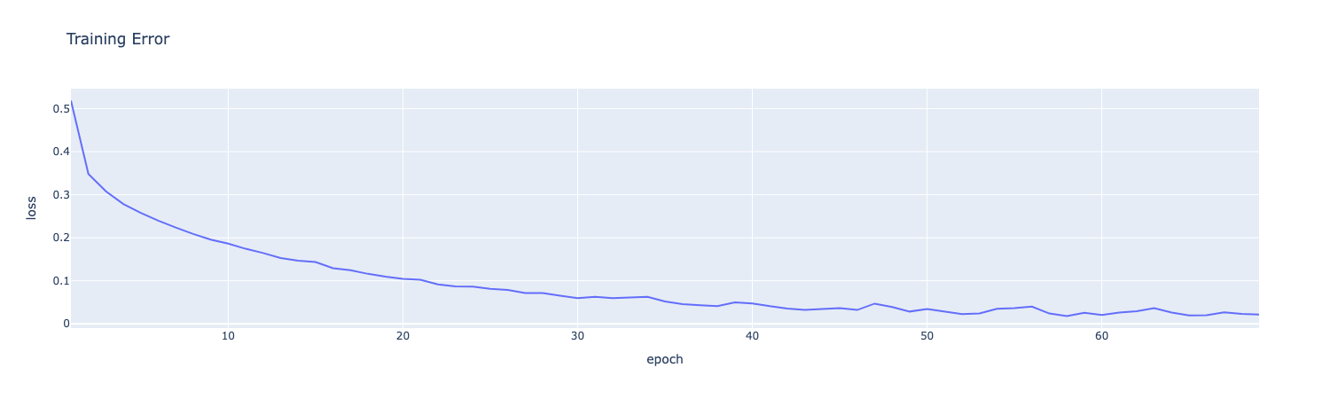
Problem 3b#
产生预测结果和Evaluation Metrics, 这里主要就是一些API的调用, 主要涉及到Sklearn.model的属性怎么用的问题
# TODO: Add the columns listed above to `train_df` and `test_df`.
train_df = train_df.copy()
test_df = test_df.copy()

train_predict=model.predict(X_train_sc)
test_predict=model.predict(X_test_sc)model.predict返回(n_samples,)的np数组, 所以他是可以直接和真实的label数组去进行比较的
train_correct=(train_predict==y_train)
test_correct=(test_predict==y_test)分类模型本质上在预测概率, 对于每个class, 给出一个prob_class, 所以model.predict_prob会给出(n_samples,n_classes)的数组, 即对于每个样本的每个潜在分类给出一个概率
train_probs=model.predict_proba(X_train_sc)
test_probs=model.predict_proba(X_test_sc)接下来还要得到每个样本的置信度, 实际上就是每个样本预测概率当中最大的那个概率, 通俗来说, 如果有十个候选类, 然后其中预测的最大概率是100%, 其他的类的概率都是0%, 那至少看起来是比较可信的
train_confidence=np.max(train_probs,axis=1)
test_confidence=np.max(test_probs,axis=1)以上均得到(n_samples,)的数组
接下来把这些贴回到原来的df上去
train_probs_list=[list(probs) for probs in train_probs]
test_probs_list=[list(probs) for probs in test_probs]

train_df['predicted_label']=train_predict
train_df['correct']=train_correct
train_df['probs']=train_probs_list
train_df['confidence']=train_confidence

test_df['predicted_label']=test_predict
test_df['correct']=test_correct
test_df['probs']=test_probs_list
test_df['confidence']=test_confidence最后算一下准确率就行了
print("--- Column Types ----")
for col in train_df.columns:
    val = train_df[col].iloc[0]
    print(f"{col}: {type(val)}")
print("-----------")


train_accuracy = train_correct.sum()/len(train_correct)
test_accuracy = test_correct.sum()/len(test_correct)

print(f"Training accuracy: {train_accuracy:.3f}")
print(f"Test accuracy: {test_accuracy:.3f}")--- Column Types ----
image: <class 'numpy.ndarray'>
label: <class 'str'>
predicted_label: <class 'str'>
correct: <class 'numpy.bool'>
probs: <class 'list'>
confidence: <class 'numpy.float64'>
-----------
Training accuracy: 0.993
Test accuracy: 0.883Problem 3c#
分组查看准确率, 只要groupby('label')['correct'].mean()就可以得到每个类的准确率, 然后再把train和test两张表concat起来, 最后用pivot把它变成宽表即可
# TODO: Calculate train and test accuracy per class
# TODO: Use class_accuracy to create a grouped bar chart of class accuracy for train and test

train_class_acc=train_df.groupby('label')['correct'].mean().reset_index()
train_class_acc['split']='train'

test_class_acc=test_df.groupby('label')['correct'].mean().reset_index()
test_class_acc['split']='test'

all_df=pd.concat([train_class_acc,test_class_acc])

class_accuracy=all_df[['split','label','correct']]
# print(class_accuracy)

class_accuracy_pivot=class_accuracy.pivot(index='label',columns='split',values='correct')
print(class_accuracy_pivot)

class_accuracy_pivot.plot(kind='bar',text_auto=True)split test train
label
Ankle boot 0.967500 0.998333
Bag 0.966667 0.999792
Coat 0.807500 0.993333
Dress 0.888333 0.995208
Pullover 0.810000 0.990208
Sandal 0.945833 0.998958
Shirt 0.737500 0.990833
Sneaker 0.932500 0.996458
T-shirt/top 0.802500 0.967083
Trouser 0.975833 0.997917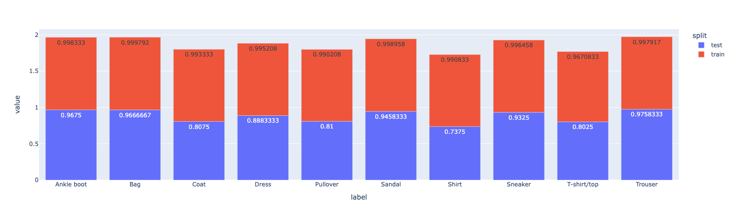
Problem 3d#
计算不同类别之间的预测效果, 首先要用np算一个10*10的confusion matrix, 行代表真实label, 列代表预测label, 每个元素代表这种预测的个数, 显然, 对角线上的元素求和就是总共预测对的数量
# Initialize confusion matrix with zeros
conf_matrix = np.zeros((len(class_names), len(class_names)), dtype=int)
class_to_idx = {class_name: idx for idx, class_name in enumerate(class_names)}

# Fill the confusion matrix by counting predictions and plot it as a heatmap
y_true=test_df['label'].values
y_pred=test_df['predicted_label'].values

true_indices = np.array([class_to_idx[label] for label in y_true])
pred_indices = np.array([class_to_idx[label] for label in y_pred])

np.add.at(conf_matrix, (true_indices, pred_indices), 1)

fig=px.imshow(conf_matrix,
                labels=dict(x="Predicted Label", y="True Label", color="Count"),
                x=class_names,
                y=class_names,
                )

fig.show()实际上就是遍历一遍真实label和预测label, 注意要把label的名字转成int, 然后对矩阵的(int,int)加一就好了
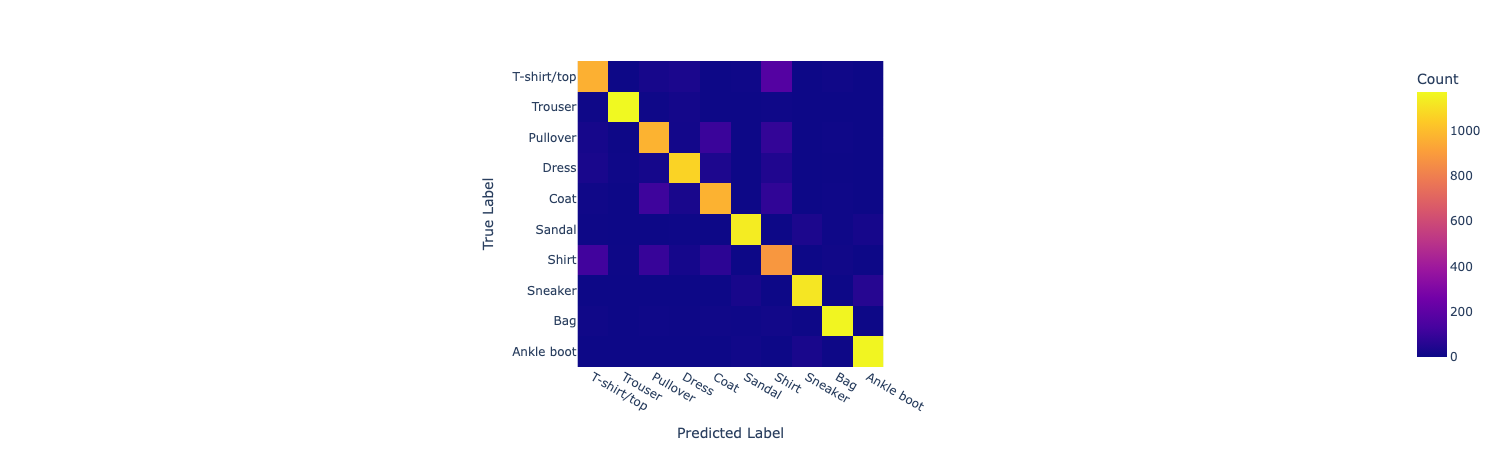
conf_matrixarray([[ 963, 0, 23, 31, 1, 4, 171, 0, 7, 0],
[ 4, 1171, 4, 15, 1, 0, 4, 0, 1, 0],
[ 20, 2, 972, 14, 102, 0, 86, 0, 4, 0],
[ 27, 5, 19, 1066, 37, 1, 43, 0, 2, 0],
[ 7, 1, 112, 28, 969, 0, 79, 0, 4, 0],
[ 2, 0, 0, 3, 0, 1135, 0, 35, 5, 20],
[ 118, 2, 96, 19, 71, 0, 885, 1, 8, 0],
[ 0, 0, 0, 0, 0, 24, 0, 1119, 1, 56],
[ 6, 1, 5, 2, 7, 4, 12, 2, 1160, 1],
[ 0, 0, 0, 0, 0, 10, 0, 27, 2, 1161]])接下来需要计算FP, FN, TP指标, 直接在这个矩阵上操作即可, 只需要注意对角线上是对的, 其他的都是错的
# Calculate accuracy from confusion matrix
accuracy_from_matrix = np.trace(conf_matrix)/np.sum(conf_matrix)
print(f"\nAccuracy calculated from confusion matrix: {accuracy_from_matrix:.3f}")

# Calculate per-class metrics from confusion matrix
per_class_metrics = []
print("\nPer-class metrics from confusion matrix:")
for i, class_name in enumerate(class_names):
    true_positives = conf_matrix[i][i]
    false_positives = np.sum(conf_matrix[:,i])-conf_matrix[i][i]
    false_negatives = np.sum(conf_matrix[i,:])-conf_matrix[i][i]
    precision = true_positives / (true_positives + false_positives) if (true_positives + false_positives) > 0 else 0.0
    recall = true_positives / (true_positives + false_negatives) if (true_positives + false_negatives) > 0 else 0.0
    per_class_metrics.append({
        'class': class_name,
        'precision': precision,
        'recall': recall
    })

pd.DataFrame(per_class_metrics)Accuracy calculated from confusion matrix: 0.883
Per-class metrics from confusion matrix: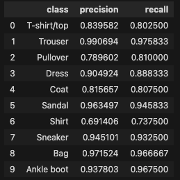
Problem 3f#
找出低置信度的预测并且plot出来
# TODO: Find the image with the lowest confidence by sorting the `confidence` column of `test_df`
least_confident = test_df.sort_values(by='confidence',ascending=True)
print("Image with lowest confidence:")
print(least_confident[['label', 'predicted_label', 'confidence', 'correct']][:3])

# Show image with lowest confidence and its predicted label
show_labels = [f"{label} (Pred: {predicted_label})" for label, predicted_label in zip(least_confident["label"].tolist(), least_confident["predicted_label"].tolist())]
fig = show_images(np.stack(least_confident["image"].tolist()), 8, ncols=4, labels=show_labels, reshape=True)
fig.show()Image with lowest confidence:
label predicted_label confidence correct
20252 Coat Shirt 0.385341 False
23752 Sneaker Ankle boot 0.395444 False
18719 Sneaker Ankle boot 0.396654 False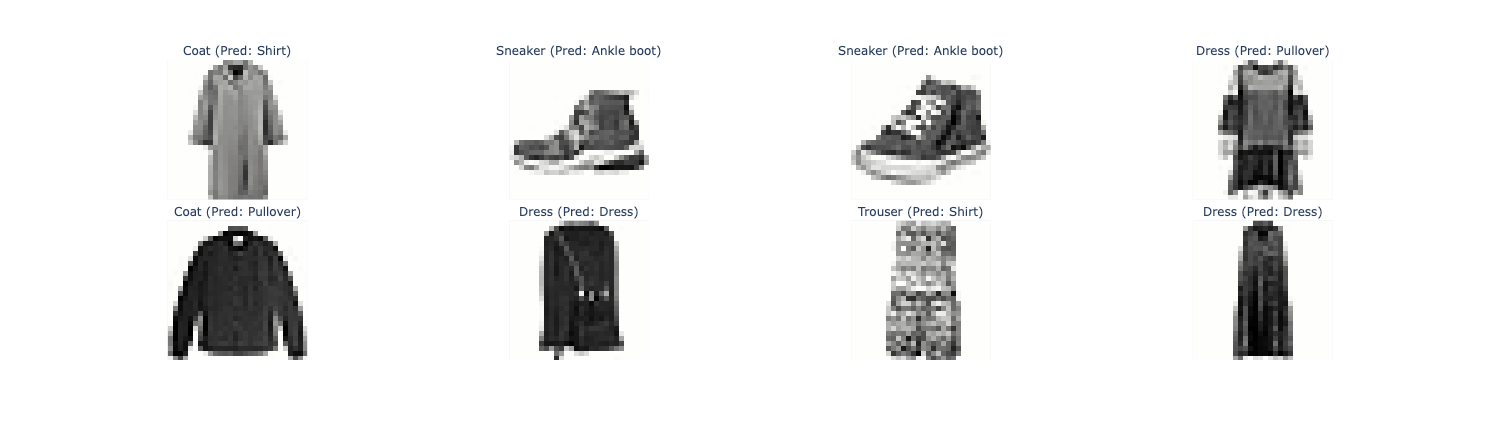
可以看到, 在置信度非常低的情况下, 很多都预测错了
Problem 3g#
找一些置信度很低但是预测对了的的Ankle boot类并画图, 非常容易, 先从test_df筛选出label == 'Ankle boot' & correct == True的, 然后用show_images画图就行了
# TODO: Visualize 10 images from the `test_set` whose true label is `Ankle boot` that the model correctly classified but with low confidence
test_df_boot = test_df[(test_df['label']=='Ankle boot')  &  (test_df['correct']==True)].sort_values(by='confidence',ascending=True).head(10)
# 将 labels 转换为列表,或者使用 .tolist()
show_labels = [f"{label} " for label in test_df_boot['label'].tolist()]
fig = show_images(np.stack(test_df_boot["image"].tolist()), 10, ncols=5, labels=show_labels, reshape=True)

fig.show()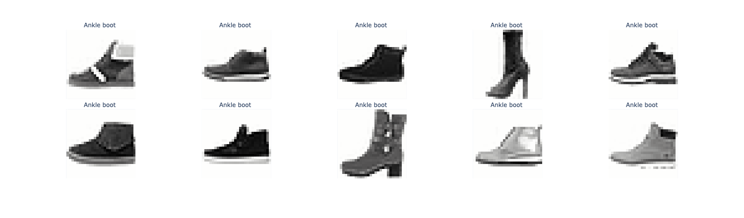
Problem 3l#
再找一些trouser类当中置信度很高但预测错误的画图, 和上面的一样, 照猫画虎即可
# TODO: Visualize 10 images from the `test_set` whose true label is `Trouser` that the model incorrectly classified as `Dress` with high confidence
test_df_trouser = test_df[(test_df['label']=='Trouser')  &  (test_df['correct']==False)].sort_values(by='confidence',ascending=False).head(10)
show_labels = [f"{label} " for label in test_df_trouser['label'].tolist()]
fig = show_images(np.stack(test_df_trouser["image"].tolist()), 10, ncols=5, labels=show_labels, reshape=True)

fig.show()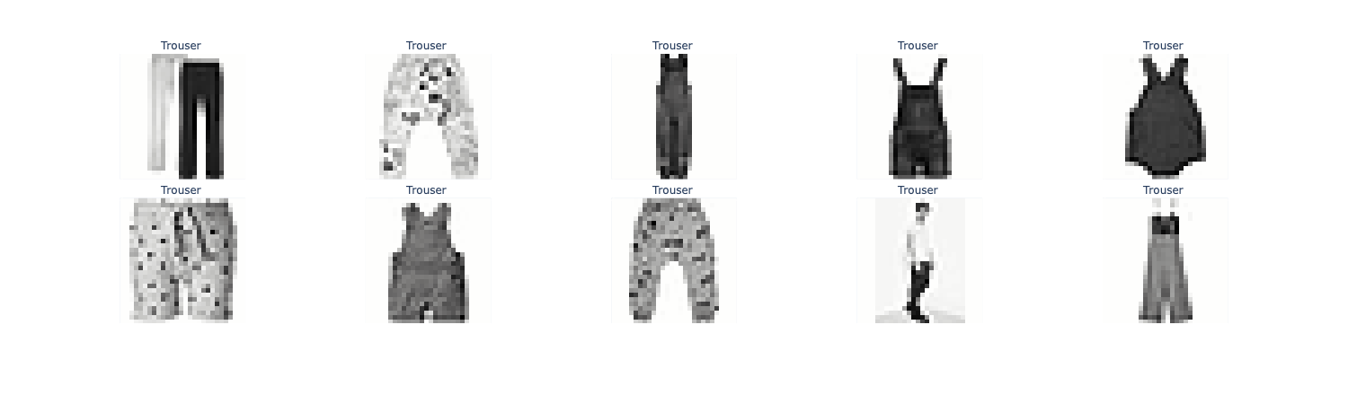
可以看到, 就算置信度很高, 也会有非常离谱的错误, 比如说把一个人分类成裤子, 从结果去理解过程, 我觉得他识别出的特征是两条裤腿
Problem 4#
这一部分作业要求我们实现各种各样的图像增强, 我个人觉得这是比较难的部分, 因为这一段的numpy调用很多, 一不小心就不记得数据处理成什么样了
首先实现一些功能函数, 在高等代数里面学过(在此致敬电子科技大学何军华老师), 很多变换(线性)都可以通过矩阵乘法来表示, 所以实现这个应用变换的函数
def apply_transformation(image, T):
    # Input: A (N, 784) image vector and a (784, 784) transformation matrix
    # Output: A (N, 784) image vector
    transformed_flat = image @ T.T
return transformed_flat.reshape(image.shape)即将变换矩阵作用在图像上, 得到新图像
接下来是一个例子, 告诉我们如何实现图像的上下颠倒
def create_vertical_flip_matrix(height=28, width=28):
    """
    Returns a (height*width, height*width) matrix that vertically flips an image
    when applied to its flattened vector. Values are 0 or 1.
    """
    N = height * width  # Total number of pixels in the image
    T = np.zeros((N, N), dtype=int)  # Initialize the transformation matrix with zeros
    for i in range(height):  # Loop over each row
        for j in range(width):  # Loop over each column
            orig_idx = i * width + j  # Compute the flattened index for the original pixel
            flipped_i = height - 1 - i  # Compute the row index after vertical flip
            flipped_idx = flipped_i * width + j  # Compute the flattened index for the flipped pixel
            # Set the corresponding entry in the transformation matrix to 1
            # This means the pixel at (i, j) moves to (flipped_i, j)
            T[flipped_idx, orig_idx] = 1
    return T

def vertical_flip(image):
    T_flip = create_vertical_flip_matrix()
return apply_transformation(image, T_flip)上下颠倒只改变行, 不改变列, 实际上就是把第i行映射到height-1-i行
test_image = np.load("test_image.npy")

flipped_image = vertical_flip(test_image)
show_images(np.stack([test_image, flipped_image]), labels=['Original', 'Flipped'], reshape=True)
这里要说一下, 这个变换矩阵T的尺寸是N*N, 其中N=height*width, 可以理解为height*width个像素点, 每个像素点从i*width + j被映射到(height-1-i)*width + j
Problem 4a#
要实现水平翻转, 依葫芦画瓢而已, 行不变, 列从j变成width - 1 - j, 所以每个元素i*width + j变到i*width + (width - 1 - j)
def create_horizontal_flip_matrix(height=28, width=28):
    """
    Returns a (height*width, height*width) matrix that horizontally flips an image
    when applied to its flattened vector. Values are 0 or 1.
    """
    N = height * width
    T = np.zeros((N, N), dtype=int)
    for i in range(height):
        for j in range(width):
            orig_idx = i * width + j
            flipped_j = width - 1 - j
            flipped_idx = i * width + flipped_j
            T[flipped_idx, orig_idx] = 1
    return T


def horizontal_flip(image):
    T_flip = create_horizontal_flip_matrix()
    return apply_transformation(image, T_flip)

flipped_image = horizontal_flip(test_image)

show_images(np.stack([test_image, flipped_image]), labels=['Original', 'Horizontal Flipped'], reshape=True)
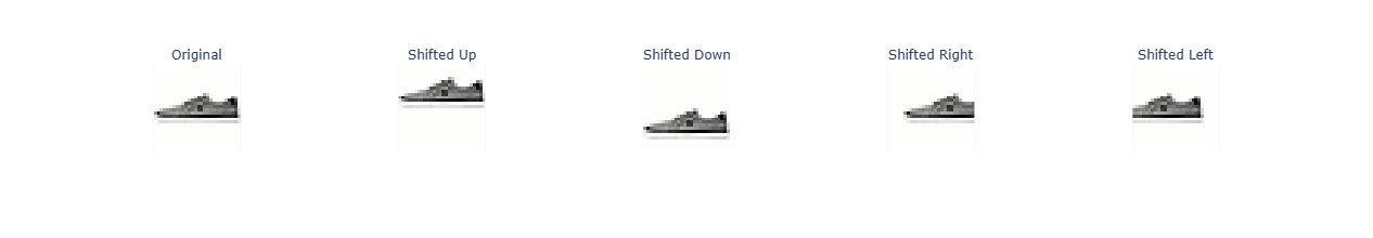
Problem 4b#
要求实现图像的Shift移动, 想象一下, 如果是水平移动, 那就是列j被映射到j + dx(先不考虑左右的符号问题), 所以每个像素点从i*width + j被映射到i*width + j + dx
这里有点小trick, 就是把x和y先flatten一下然后再移动
def create_shift_matrix(dx, dy, height=28, width=28):
    """
    Create a transformation matrix for shifting an image by dx pixels horizontally and dy pixels vertically.

    Args:
        dx (int): Number of pixels to shift horizontally.
        dy (int): Number of pixels to shift vertically.
        height (int): Height of the image.
        width (int): Width of the image.

    Returns:
        np.ndarray: A (height*width, height*width) transformation matrix for shifting.
    """
    N = height * width
    T = np.zeros((N, N))
    yy, xx = np.meshgrid(np.arange(height), np.arange(width), indexing='ij')
    yy_flat = yy.ravel()
    xx_flat = xx.ravel()

    y_shift = yy_flat + dy
    x_shift = xx_flat + dx

    valid = (
        (y_shift >= 0) & (y_shift < height) &
        (x_shift >= 0) & (x_shift < width)
    )

    src = yy_flat[valid] * width + xx_flat[valid]
    dst = y_shift[valid] * width + x_shift[valid]

    T[dst, src] = 1.0

    return T


def shift_image(image, dx, dy):
    """
    Shift an image by dx pixels horizontally and dy pixels vertically.

    Args:
        image (np.ndarray): Flattened image array of shape (height*width,).
        dx (int): Number of pixels to shift horizontally.
        dy (int): Number of pixels to shift vertically.

    Returns:
        np.ndarray: Shifted image as a flattened array.
    """
    T = create_shift_matrix(dx, dy)
    return apply_transformation(image, T)

shifted_right_image = shift_image(test_image, 5, 0)
shifted_left_image = shift_image(test_image, -5, 0)
shifted_up_image = shift_image(test_image, 0, -5)
shifted_down_image = shift_image(test_image, 0, 5)

all_images = np.stack([test_image, shifted_up_image, shifted_down_image, shifted_right_image, shifted_left_image])
plot_labels = ['Original', 'Shifted Up', 'Shifted Down', 'Shifted Right', 'Shifted Left']
show_images(all_images, labels=plot_labels, reshape=True)注意这上面的xx yy都有height*weight个元素, 他们本质上是所有元素的列坐标和行坐标, 所以说被flatten以后, 比如说xx_flat + dx就是对所有的列坐标都加上dx, 然后后面再用形如i * width + height的方式来还原
Problem 4c#
要求实现一个类似于卷积核的东西, 关键是要搞清楚src_idx和dst_idx之间的关系, 还要搞清楚这个矩阵T的含义, 矩阵T有weight*height行, 每一行对应原矩阵的一个点, 而每一行的weight*height个点对应的是原矩阵的这一个点对总共的weight*height个点产生的影响
举个例子:
0 1 2
3 4 5
6 7 8原有矩阵是这样, 那么T的第一行就应该是:
[1/4, 1/4, 0, 1/4, 1/4, 0, 0, 0, 0 ],这一行有9个点, 代表的就是对原矩阵9个点的影响, 我们假设kernel_size = 3, 那么生成的(0,0)处的元素应当是(0+1+3+4)/4, 也就是把原矩阵Flatten成行了之后和这一行(转置成列)做内积, 而那些没被影响的点, 在这一行里的数值自然就是0了
def create_blur_matrix(kernel_size=3, height=28, width=28):
    """
    Create a transformation matrix T that applies a uniform mean blur using a centered, odd-sized square sliding window.

    For each output pixel (i, j):
      1) Place a `kernel_size × kernel_size` window centered at (i, j).
      2) If the window is outside the image, then it will have fewer neighbors (only average the pixels that exist)

    Args:
        kernel_size (int): Size of the square kernel (must be odd).
        height (int): Height of the image.
        width (int): Width of the image.

    Returns:
        np.ndarray: A (height*width, height*width) transformation matrix for blurring.
    """
    N = height * width
    T = np.zeros((N, N))
    pad = kernel_size // 2
    kernel_area = kernel_size * kernel_size
    # Each pixel contributes equally to a kernel's neighborhood
    for i in range (height):
        for j in range (width):
            col_start=max(0,j-pad)
            row_start=max(0,i-pad)
            col_end=min(width-1,j+pad)
            row_end=min(height-1,i+pad)

            valid_count=(row_end-row_start+1)*(col_end-col_start+1)
            arg_value=1.0/valid_count

            dst_idx=i*width+j
            for r in range(row_start,row_end+1):
                for c in range(col_start,col_end+1):
                    src_idx=r*width+c
                    T[dst_idx,src_idx]=arg_value
return T可以看到一个i和j确定了唯一的dst_idx, 这个变量名没太起好, 这其实是原矩阵的(i,j)点, 那么在T当中他要占一整行, 而一整行每个被影响的点都是1/count, 影响不到的(窗口外的)自然就是0了
应用并画图
def blur_image(image, kernel_size=3):
    """
    Apply a blur transformation to a flattened image array or a batch of flattened images.

    Args:
        image (np.ndarray): Flattened image array of shape (height*width,) or batch of images (N, height*width).
        kernel_size (int): Size of the square kernel to use for blurring.

    Returns:
        np.ndarray: Blurred image(s) as a flattened array or batch of arrays.
    """
    T = create_blur_matrix(kernel_size)
    return apply_transformation(image, T)

blurred_1x1 = blur_image(test_image, kernel_size=1)
blurred_3x3 = blur_image(test_image, kernel_size=3)
blurred_5x5 = blur_image(test_image, kernel_size=5)

blurred_images = [test_image, blurred_1x1, blurred_3x3, blurred_5x5]
blurred_labels = ['Original', 'Blur 1x1', 'Blur 3x3', 'Blur 5x5']

show_images(blurred_images, labels=blurred_labels, reshape=True)Problem 4d#
要求实现图像旋转矩阵
这里的核心是根据生成的旋转变换2*2矩阵
根据一年级的解析几何课程知识(在此致敬电子科技大学余时伟老师), 点(x,y)如果围绕原点旋转得到的(x',y')满足:
更一般的如果是围绕(x_0,y_0)进行旋转, 只要搞清楚本质上是向量再旋转就行, 所以满足:
def create_rotation_matrix(theta, height=28, width=28):
"""
Create a transformation matrix for rotating an image by theta degrees.
Args:
theta (float): Angle of rotation in degrees.
height (int): Height of the image.
width (int): Width of the image.
Returns:
np.ndarray: A (height*width, height*width) transformation matrix for rotating.
"""
# Convert theta from degrees to radians
theta = np.deg2rad(theta)
N = height * width
T = np.zeros((N, N))
center_i = (height - 1) / 2.0
center_j = (width - 1) / 2.0
cos_theta = np.cos(theta)
sin_theta = np.sin(theta)
for src_i in range(height):
for src_j in range(width):
src_i_centered = src_i - center_i
src_j_centered = src_j - center_j
# 旋转(逆时针旋转theta)
dst_i_centered = src_i_centered * cos_theta - src_j_centered * sin_theta
dst_j_centered = src_i_centered * sin_theta + src_j_centered * cos_theta
# 平移回去
dst_i = dst_i_centered + center_i
dst_j = dst_j_centered + center_j
# 取整并检查边界
dst_i_int = int(np.round(dst_i))
dst_j_int = int(np.round(dst_j))
if 0 <= dst_i_int < height and 0 <= dst_j_int < width:
src_idx = src_i * width + src_j
dst_idx = dst_i_int * width + dst_j_int
T[dst_idx, src_idx] = 1.0
return T
def rotate_image(image, theta):
"""
Apply a rotation transformation to a flattened image array or a batch of flattened images.
Args:
image (np.ndarray): Flattened image array of shape (height*width,) or batch of images (N, height*width).
theta (float): Angle of rotation in degrees.
Returns:
np.ndarray: Rotated image(s) as a flattened array or batch of arrays.
"""
T = create_rotation_matrix(theta)
return apply_transformation(image, T)
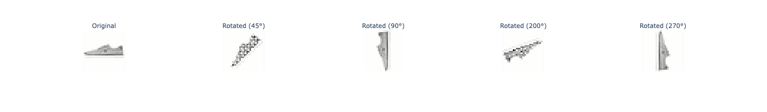
# rotate with matrix
rotated_45 = rotate_image(test_image, 45)
rotated_90 = rotate_image(test_image, 90)
rotated_200 = rotate_image(test_image, 200)
rotated_270 = rotate_image(test_image, 270)
# visualize original and 4 augmentations in plotly image grid
all_images = np.stack([test_image, rotated_45, rotated_90, rotated_200, rotated_270])
plot_labels = ['Original', 'Rotated (45°)', 'Rotated (90°)', 'Rotated (200°)', 'Rotated (270°)']
show_images(all_images, labels=plot_labels, reshape=True)这里的映射关系就是:
(i, j) -> (dst_i, dst_j)再构造出两边的src_idx和dst_idx即可, 注意这个T在apply_transformation的时候要转置的, 所以在填充T的时候永远是T[dst_idx, src_idx], 转置之后就变成T[src_idx, dst_idx]
Problem 4e#
要求实现逆旋转变换和双线性插值, 首先考虑逆变换(x_0,y_0)到(x,y)
def create_bilinear_rotation_matrix(theta, height=28, width=28):
    """
    Create a (height*width, height*width) matrix that applies bilinear interpolation
    for rotating a flattened image by theta degrees.
    Each row of the matrix gives the weights for the input pixels that contribute to each output pixel.

    Args:
        theta (float): Angle of rotation in degrees.
        height (int): Height of the image.
        width (int): Width of the image.

    Returns:
        np.ndarray: A (height*width, height*width) transformation matrix for rotating.
    """
    theta = np.deg2rad(theta)
    N = height * width
    T = np.zeros((N, N))
    center_i = (height - 1) / 2.0
    center_j = (width - 1) / 2.0
    cos_theta = np.cos(-theta)
    sin_theta = np.sin(-theta)

    for i in range(height):  # Loop over rows of the output image
        for j in range(width):  # Loop over columns of the output image
            output_idx = i * width + j

            # Translate output pixel to be relative to the center
            centered_j = j - center_j
            centered_i = i - center_i

            # Apply the inverse rotation to find the original pixel coordinates
            original_j_rotated = centered_j * cos_theta - centered_i * sin_theta
            original_i_rotated = centered_j * sin_theta + centered_i * cos_theta

            # Translate back to original image coordinates
            original_j = original_j_rotated + center_j
            original_i = original_i_rotated + center_i

            # Bilinear interpolation
            # Find the 4 nearest neighbor pixels
            j_floor = int(np.floor(original_j))
            i_floor = int(np.floor(original_i))
            j_ceil = int(np.ceil(original_j))
            i_ceil = int(np.ceil(original_i))

            # Calculate the fractional distances
            dj = original_j - j_floor
            di = original_i - i_floor

            # Define the weights
            w_tl = (1 - dj) * (1 - di)  # Top-left
            w_tr = dj * (1 - di)      # Top-right
            w_bl = (1 - dj) * di      # Bottom-left
            w_br = dj * di          # Bottom-right

            # Get the indices of the 4 neighbors, handling boundaries by setting weight to 0
            neighbors = []
            weights = []

            # Top-left neighbor
            if 0 <= i_floor < height and 0 <= j_floor < width:
                neighbors.append(i_floor * width + j_floor)
                weights.append(w_tl)

            # Top-right neighbor
            if 0 <= i_floor < height and 0 <= j_ceil < width:
                neighbors.append(i_floor * width + j_ceil)
                weights.append(w_tr)

            # Bottom-left neighbor
            if 0 <= i_ceil < height and 0 <= j_floor < width:
                neighbors.append(i_ceil * width + j_floor)
                weights.append(w_bl)

            # Bottom-right neighbor
            if 0 <= i_ceil < height and 0 <= j_ceil < width:
                neighbors.append(i_ceil * width + j_ceil)
                weights.append(w_br)

            # Assign the weighted sum to the output pixel in the transformation matrix
            for neighbor_idx, weight in zip(neighbors, weights):
                T[output_idx, neighbor_idx] = weight
return T首先这里遍历的其实是输出的image了, 不过尺寸还是一样的, 只要应用上面的矩阵变换就能得到原来的original_j和original_i, 也就是变换前的y和x
注意由于是三角函数的数值变换, 这个y和x不一定是整数, 所以我们找它周边的四个点做双线性插值
# Bilinear interpolation
# Find the 4 nearest neighbor pixels
j_floor = int(np.floor(original_j))
i_floor = int(np.floor(original_i))
j_ceil = int(np.ceil(original_j))
i_ceil = int(np.ceil(original_i))

# Calculate the fractional distances
dj = original_j - j_floor
di = original_i - i_floor然后计算四个权重, 以竖着的距离为例, x到i_floor的距离是di, x到i_ceil的距离是1-di, 这是因为i_floor到i_ceil的距离是1
# Define the weights
w_tl = (1 - dj) * (1 - di)  # Top-left
w_tr = dj * (1 - di)      # Top-right
w_bl = (1 - dj) * di      # Bottom-left
w_br = dj * di # Bottom-right接下来, 遍历这四个邻居点并且添加权重, 注意在一次遍历当中output_idx是已经被固定了的, 然后在T的属于output_idx的那一行里面, 至多有四个不为0的weight(如果neighbor出格了就不要了)
# Top-left neighbor
if 0 <= i_floor < height and 0 <= j_floor < width:
    neighbors.append(i_floor * width + j_floor)
    weights.append(w_tl)

# Top-right neighbor
if 0 <= i_floor < height and 0 <= j_ceil < width:
    neighbors.append(i_floor * width + j_ceil)
    weights.append(w_tr)

# Bottom-left neighbor
if 0 <= i_ceil < height and 0 <= j_floor < width:
    neighbors.append(i_ceil * width + j_floor)
    weights.append(w_bl)

# Bottom-right neighbor
if 0 <= i_ceil < height and 0 <= j_ceil < width:
    neighbors.append(i_ceil * width + j_ceil)
    weights.append(w_br)

# Assign the weighted sum to the output pixel in the transformation matrix
for neighbor_idx, weight in zip(neighbors, weights):
T[output_idx, neighbor_idx] = weight应用更改
def rotate_image_bilinear(image, theta):
    """
    Rotate an image using bilinear interpolation.

    Args:
        image (np.ndarray): Flattened image array of shape (height*width,) or batch of images (N, height*width).
        theta (float): Angle of rotation in degrees.

    Returns:
        np.ndarray: Rotated image as a flattened array.
    """
    T = create_bilinear_rotation_matrix(theta)
    return apply_transformation(image, T)

# rotate with matrix
rotated = rotate_image(test_image, 45)
rotated_interpolated = rotate_image_bilinear(test_image, 45)

all_images = np.stack([test_image, rotated, rotated_interpolated])
plot_labels = ['Original',  'Rotated 45°', 'Rotated 45° (Bilinear)']
show_images(all_images, labels=plot_labels, reshape=True)
Problem 4f#
实现复合变换, 假如我们有很多变换矩阵T在一个列表里面, 我们只需要遍历这个列表然后每次进行矩阵相乘就好了
def compose_transforms(*Ts):
  """
  Compose linear image transforms (each 784x784).
  Inputs:
    Ts: list of transformation matrices
  Returns:
    T_total: composition of all input transformations
  """
  T_total = Ts[0]
  for T in Ts[1:]:
    T_total = np.dot(T, T_total)  # 注意:T @ T_total,不是 T_total @ T
return T_total例如先旋转再模糊化处理:
def rotate_then_blur(image, theta, kernel_size):
  """
  Rotate an image by theta degrees (without bilinear interpolation) and then blur it with a kernel of size kernel_size.
  """


  Rotate_Matrix=create_rotation_matrix(theta,height=28,width=28)
  Blur_Matrix=create_blur_matrix(kernel_size=kernel_size,height=28,width=28)

  T=compose_transforms(Rotate_Matrix,Blur_Matrix)


return apply_transformation(image,T)以及先平移, 再旋转, 再模糊化处理
def shift_then_rotate_then_blur(image, dx, dy, theta, kernel_size):
  """
  Shift an image by (dx, dy), then rotate it by theta degrees (without bilinear interpolation), and then blur it with a kernel of size kernel_size.
  """
  Shift_Matrix=create_shift_matrix(dx,dy,height=28,width=28)
  Rotate_Matrix=create_rotation_matrix(theta,height=28,width=28)
  Blur_Matrix=create_blur_matrix(kernel_size,height=28,width=28)
  T=compose_transforms(Shift_Matrix,Rotate_Matrix,Blur_Matrix)
return apply_transformation(image,T)rotated_blurred_image = rotate_then_blur(test_image, 45, 3)
# shifted_rotated_blurred_image = shift_then_rotate_then_blur(test_image, 1, -4, 200, 5)
shifted_rotated_blurred_image = shift_then_rotate_then_blur(test_image, 5, 5, 45, 5)
all_images = np.stack([test_image, rotated_blurred_image, shifted_rotated_blurred_image])
plot_labels = ['Original', 'Rotated 45° and Blurred 2x2', 'Shifted 5, Rotated 45° and Blurred 2x2']
show_images(all_images, labels=plot_labels, reshape=True)
这个问题的测试没A过, 但是也没有看出来有什么问题
Problem 4h#
写一个接口来应用这些更改, 不需要什么技巧, 直接把变换的类型和参数存起来, 然后for循环一个一个应用即可
# Test augmentation functions on a few examples
test_images = np.stack(test_df['image'])
test_labels = test_df['label']

shift_inputs = [(5, 0), (-5, 0), (0, 5), (0, -5)]
rotate_inputs = [45, 90, 200]
blur_inputs = [3, 5]
rotate_blur_inputs = [(45, 3), (90, 5)]
shift_rotate_blur_inputs = [((5, 0), 45, 3), ((-5, 0), 90, 5)]

augmented_data = []
# Randomly sample 100 datapoints from test_images
sample_idx = np.random.choice(len(test_images), 100, replace=False)
test_images_sample = test_images[sample_idx]
test_labels_sample = np.array(test_labels)[sample_idx]

# TODO: Apply the augmentation functions we just created (shift, blur, rotate w/ bilinear, rotate then blur, shift then rotate then blur) to every image from test_images_sample
# use the inputs defined above to apply the augmentations
# Save the augmented images in a new DataFrame aug_df
def add_augmented_sample(img, label, orig_idx, aug_name, aug_type, transform_fn):
    augmented_data.append({
        'original_idx': orig_idx,
        'augmentation': aug_name,
        'image': transform_fn(img).copy(),
        'label': label,
        'type': aug_type
    })


for orig_idx, img, label in zip(sample_idx, test_images_sample, test_labels_sample):
    for dx, dy in shift_inputs:
        add_augmented_sample(
            img, label, orig_idx,f'shift_{dx}_{dy}', 'shift',
            lambda x, dx=dx, dy=dy: shift_image(x, dx, dy)
        )
    for theta in rotate_inputs:
        add_augmented_sample(
            img, label, orig_idx,f'rotate_bilinear_{theta}', 'rotate',
            lambda x, theta=theta: rotate_image_bilinear(x, theta)
        )
    for k in blur_inputs:
        add_augmented_sample(
            img, label, orig_idx,f'blur_{k}x{k}', 'blur',
            lambda x, k=k: blur_image(x, kernel_size=k)
        )
    for theta, k in rotate_blur_inputs:
        add_augmented_sample(
            img, label, orig_idx,f'rotate_{theta}_blur_{k}', 'rotate_blur',
            lambda x, theta=theta, k=k: rotate_then_blur(x, theta, k)
        )
    for (shift_pair, theta, k) in shift_rotate_blur_inputs:
        dx, dy = shift_pair
        add_augmented_sample(
            img, label, orig_idx,f'shift_{dx}_{dy}_rotate_{theta}_blur_{k}', 'shift_rotate_blur',
            lambda x, dx=dx, dy=dy, theta=theta, k=k: shift_then_rotate_then_blur(x, dx, dy, theta, k)
        )


aug_df = pd.DataFrame(augmented_data)

# TODO: Select an image and visualize it with all the augmentations applied to it
example_image = test_images_sample[0]

example_variants = [('original', example_image)]
for dx, dy in shift_inputs:
    example_variants.append((f'shift_{dx}_{dy}', shift_image(example_image, dx, dy)))
for theta in rotate_inputs:
    example_variants.append((f'rot_bilin_{theta}', rotate_image_bilinear(example_image, theta)))
for k in blur_inputs:
    example_variants.append((f'blur_{k}x{k}', blur_image(example_image, kernel_size=k)))
for theta, k in rotate_blur_inputs:
    example_variants.append((f'rot_{theta}_blur_{k}', rotate_then_blur(example_image, theta, k)))
for (shift_pair, theta, k) in shift_rotate_blur_inputs:
    dx, dy = shift_pair
    example_variants.append((f'shift_{dx}_{dy}_rot_{theta}_blur_{k}',
                             shift_then_rotate_then_blur(example_image, dx, dy, theta, k)))

example_imgs = np.stack([img for _, img in example_variants])
example_labels = [name for name, _ in example_variants]

fig = show_images(example_imgs, ncols=4, labels=example_labels, reshape=True)
fig.show()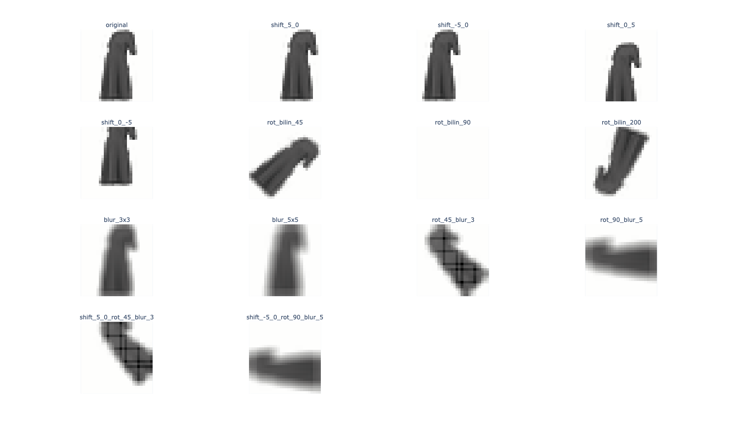
Problem 4i#
把之前训练好的那个分类器在增强数据上测试, 评测一下效果, 也就是预处理一下数据, 把格式调成适配model的样子, 最后把效果画个图就好了
from sklearn.metrics import accuracy_score


def evaluate_augmented_data(aug_df, clf):
    records = []

    for aug_name, group in aug_df.groupby("augmentation"):
        # 将图像堆叠成 3D/4D 数组,再 reshape 成模型需要的形状
        images = np.stack(group["image"].to_numpy())
        n_samples = images.shape[0]
        X = images.reshape(n_samples, -1)

        # 若模型需要标准化,这里先拟合再变换(或对训练集拟合后在此仅 transform)
        scaler = StandardScaler()
        X_scaled = scaler.fit_transform(X)

        y_true = group["label"].to_numpy()
        y_pred = clf.predict(X_scaled)
        acc = accuracy_score(y_true, y_pred)

        records.append({
            "augmentation": aug_name,
            "accuracy": acc,
            "type": group["type"].iloc[0]
        })

    return pd.DataFrame(records)


aug_performance = evaluate_augmented_data(aug_df, model)
aug_performance = aug_performance.sort_values("accuracy", ascending=False).reset_index(drop=True)
aug_performance
# Visualize performance: sort by accuracy, color by augmentation type (blur, rotate, shift, none)

fig = px.bar(
    aug_performance,
    x="augmentation",
    y="accuracy",
    color="type",
    title="Classifier Accuracy on Augmented Data"
)
fig.update_layout(xaxis_title="Augmentation", yaxis_title="Accuracy")
fig.show()
<img src="/images/189_hw1/189_hw1_20.png" alt="label_plot" />